Python

Motivation

Python has developed into an (almost) indispensable tool in computational and engineering sciences, in particular in combination with Jupyter notebooks [Per15, Per18].

Python offers an intuitive syntax with a high degree of code readability and it is used for everything from simple scripting and fast prototyping to large-scale projects.

Python is open source and free for use and distribution. It is available for all relevant platforms, including

• Linux

• MacOS

• Windows

Important modules

Python code is typically written in the form of functions that are stored in libraries (or modules) and made available with the import statement.

Modules of specific concern in this course include

• NumPy introduces multi-dimensional arrays and provides efficient array operations

• SciPy provides mathematical algorithms and convenience functions built on NumPy

• Matplotlib is a visualization library in Python for plotting arrays

• VeloxChem is a quantum chemistry program for molecular simulations.

Documentation

The amount of Python documentation is vast and so is the community of module contributers. If you are in search of the solution to an isolated task or problem, there is a great chance that someone has contributed an efficient and stable implementation on the web.

• The official course book is An Introduction to Python Programming for Scientists and Engineers [LAMCE+22].

• One of many alternative is the book titled A Whirlwind Tour of Python authored by Jake VanderPlas as it provides a short, clear, and to-the-point presentation [Van16].

• If you have some experience and rather benefit from a more reference-oriented documentation, a recommended source is W3Schools.

• If you find watching tutorial videos useful, the series made by Corey Schafer is recommended. Below is one example from this series.

Some necessities

Iterations

A for loop is used for iterating over an iterable object (such as a list, dictionary, or string).

A “standard” loop is accomplished with the range function. The range function returns an iterable sequence of numbers, starting from 0 by default, and increments by 1 (by default), and ends at a specified number.

for i in range(5):
    print(i)

0
1
2
3
4

Data types

Basic Python data types include integer, float, string, list, and dictionary.

i = 10     # integer
x = 3.1415 # float
s = 'text' # string

a_list = [x, [1,2,3]] # list
b_dict = {'first': s, 'second': a_list} # dictonary

print('Elements in list:')
for i, a in enumerate(a_list):
    print(i, a, a_list[i])

print('Elements in dictionary:')
for key in b_dict.keys():
    print('Key, value:', key, b_dict[key])

Elements in list:
0 3.1415 3.1415
1 [1, 2, 3] [1, 2, 3]
Elements in dictionary:
Key, value: first text
Key, value: second [3.1415, [1, 2, 3]]

The object type is revealed by the type function.

type(a_list)

list

Note

A Python list with \(N\) elements is indexed from 0 to \((N-1)\).

Conditions

Python supports the usual logical conditions:

• Equal: a == b

• Not Equal: a != b

• Less than: a < b

• Less than or equal to: a <= b

• Greater than: a > b

• Greater than or equal to: a >= b

These conditions are typically used in conjunction with if statements.

alcohols = {
    'cyclohexanol': {'formula': 'C6H11OH',
                     'boiling point': 162 },
    'ethanol': {'formula': 'CH3-CH2OH',
                'boiling point': 78 },
    'isopropanol': {'formula': 'CH3-CHOH-CH3',
                    'boiling point': 80 },
    'methanol': {'formula': 'CH3OH',
                 'boiling point': 65 },
    'phenylmethanol': {'formula': 'C6H5-CH2OH',
                       'boiling point': 205 },
}

lowest_bp = 9999
for key in alcohols.keys():
    if alcohols[key]['boiling point'] < lowest_bp:
        alc_with_lowest_bp = key
        lowest_bp = alcohols[key]['boiling point']

print(alc_with_lowest_bp.capitalize(), 'has the lowest boiling point.')
print('It has chemical formula:', alcohols[alc_with_lowest_bp]['formula'])
print('It has a boiling point of', lowest_bp, 'degrees Celsius.')

Methanol has the lowest boiling point.
It has chemical formula: CH3OH
It has a boiling point of 65 degrees Celsius.

Arrays with NumPy

Arrays (such as vectors and matrices) should be represented as objects of the NumPy ndarray class. Array creation can be performed in numerous ways. Two ways to create a NumPy array from a Python list are given below.

import numpy as np

a = np.array([[1,2,3],[4,5,6],[7,8,9]])
print('Alternative 1:\n', a)

a = np.array([1,2,3,4,5,6,7,8,9]).reshape((3,3))
print('Alternative 2:\n', a)

Alternative 1:
 [[1 2 3]
 [4 5 6]
 [7 8 9]]
Alternative 2:
 [[1 2 3]
 [4 5 6]
 [7 8 9]]

There are several predeifined arrays, all available for different data types.

a = np.zeros((3,3), dtype='int')
print('Zero matrix:\n', a)

a = np.ones((3,3), dtype='float')
print('One matrix:\n', a)

a = np.identity(3, dtype='complex')
print('Identity matrix:\n', a)

Zero matrix:
 [[0 0 0]
 [0 0 0]
 [0 0 0]]
One matrix:
 [[1. 1. 1.]
 [1. 1. 1.]
 [1. 1. 1.]]
Identity matrix:
 [[1.+0.j 0.+0.j 0.+0.j]
 [0.+0.j 1.+0.j 0.+0.j]
 [0.+0.j 0.+0.j 1.+0.j]]

Array operations

Array operations should be performed with NumPy routines. The NumPy array operation routines are based on optimized libraries that enable multi-thread execution with use of OpenMP. On a computer equipped with an Intel processor, the underlying library for NumPy is normally chosen as the Math Kernel Library (MKL). Never feel tempted to use for loops as the performance is tyically orders of magnitude slower. The two most important Numpy array operations are

• dot(a,b): vector dot product

• matmul(a,b): matrix mulitplication

A comparison of the use of matmul and for loops for the multiplication of two matrices of dimension 100\(\times\)100 shows the following execution times (in ms).

import time

# Fixing random state for reproducibility
np.random.seed(20210802)

N = 100

a = np.random.rand(N*N).reshape((N,N))
b = np.random.rand(N*N).reshape((N,N))

ti = time.time()

c = np.matmul(a,b)

tf = time.time()

print(f'  matmul: {(tf - ti) * 1000:10.4f} (ms)')

ti = time.time()

for i in range(N):
    for j in range(N):
        for k in range(N):
            c[i,j] = a[i,k] * b[k,j]

tf = time.time()

print(f'for loop: {(tf - ti) * 1000:10.4f} (ms)')

  matmul:     0.4182 (ms)

for loop:   289.3832 (ms)

Classes and object-oriented programming

Python naturally invites to good software engineering practices in terms of object-oriented programming. Almost everything in Python is an object, with its properties and methods and a class is like an object constructor, or a “blueprint” for creating objects known as instances of the class.

It cannot be overemphasized that the use of object-oriented programming is highly enabling for code sharing and team development, and it is strongly recommended to adopt these practices.

As an example, we implement a class Triangle with a method area and attributes base and height.

class Triangle:
    def __init__(self, base, height):
        self.base = base
        self.height = height
        
    def area(self):
        A = self.base * self.height / 2
        return A

Note

The instance reference is automatically passed as the first argument to the methods. By convention, this argument should be recieved as a parameter named self.

The __init__ method is executed every time a new instance of the class is created.

It is a common practice to store the code of classes in separate library files (or modules) with the file extension *.py. In this case, we can imagine that we store the Triangle class together with several other geometric objects into a module named geometry.py after which these would be readily available from other modules by means of an import statement:

import geometry as gm

where gm is an optional shorter name reference of your choice.

The user of such an encapsulated module need not be concerned about the details of the code which is the key enabling factor for code-sharing. We define an instance of this class according to

t = gm.Triangle(3, 5)

and execute the function that calculates the area and print out the result as follows

print("Area:", t.area())

If the class is kept in the notebook the import statement is obviously not needed and we instead access the instance attributes and methods as follows

t = Triangle(3, 5)         # class instance

print('Base:', t.base)     # instance attribute
print('Height:', t.height) # instance attribute

print('Area:', t.area())   # instance method

Base: 3
Height: 5
Area: 7.5

Plotting with Matplotlib

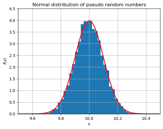
Let us use NumPy to generate an array of random numbers distributed according to the Gaussian distribution

\[ f(x) = \frac{1}{\sqrt{2\pi\sigma^2}} e^{-(x-\mu)^2 / (2\sigma^2)} \]

import numpy as np

# Fixing random state for reproducibility
np.random.seed(20210722)

mu, sigma = 10, 0.1 # mean and standard deviation
s = np.random.normal(mu, sigma, 5000) # return a NumPy array

print('Object type:', type(s))
print('Number of values:', len(s))
print(f'Mean value: {np.mean(s) : .4f}')
print(f'Standard deviation: {np.std(s) : .4f}')

Object type: <class 'numpy.ndarray'>
Number of values: 5000
Mean value:  10.0002
Standard deviation:  0.0996

We use Matplotlib to plot a histogram of the density distribution of the random numbers and compared it to the analytical Gaussian distribution function \(f(x)\) given above.

import matplotlib.pyplot as plt

counts, x, patches = plt.hist(s, bins=50, range=(9.5,10.5), density=True)

f = 1 / ( sigma * np.sqrt(2 * np.pi) ) * np.exp( - (x - mu)**2 / (2 * sigma**2) )

plt.plot(x, f, linewidth=2, color='r')

plt.grid(True)
plt.setp(plt.gca(), xlim=(9.5,10.5), ylim=(0,4.5))
plt.title('Normal distribution of pseudo random numbers')
plt.xlabel(r'$x$')
plt.ylabel(r'$f(x)$')

# save the figure in your favorite format
#plt.savefig('figname.pdf')
#plt.savefig('figname.png')

plt.show()

Python help function

The Python help function is used to display the documentation of modules, functions, classes, keywords etc.

help(plt.hist)

Help on function hist in module matplotlib.pyplot:

hist(x: 'ArrayLike | Sequence[ArrayLike]', bins: 'int | Sequence[float] | str | None' = None, *, range: 'tuple[float, float] | None' = None, density: 'bool' = False, weights: 'ArrayLike | None' = None, cumulative: 'bool | float' = False, bottom: 'ArrayLike | float | None' = None, histtype: "Literal['bar', 'barstacked', 'step', 'stepfilled']" = 'bar', align: "Literal['left', 'mid', 'right']" = 'mid', orientation: "Literal['vertical', 'horizontal']" = 'vertical', rwidth: 'float | None' = None, log: 'bool' = False, color: 'ColorType | Sequence[ColorType] | None' = None, label: 'str | Sequence[str] | None' = None, stacked: 'bool' = False, data=None, **kwargs) -> 'tuple[np.ndarray | list[np.ndarray], np.ndarray, BarContainer | Polygon | list[BarContainer | Polygon]]'
    Compute and plot a histogram.

    This method uses `numpy.histogram` to bin the data in *x* and count the
    number of values in each bin, then draws the distribution either as a
    `.BarContainer` or `.Polygon`. The *bins*, *range*, *density*, and
    *weights* parameters are forwarded to `numpy.histogram`.

    If the data has already been binned and counted, use `~.bar` or
    `~.stairs` to plot the distribution::

        counts, bins = np.histogram(x)
        plt.stairs(counts, bins)

    Alternatively, plot pre-computed bins and counts using ``hist()`` by
    treating each bin as a single point with a weight equal to its count::

        plt.hist(bins[:-1], bins, weights=counts)

    The data input *x* can be a singular array, a list of datasets of
    potentially different lengths ([*x0*, *x1*, ...]), or a 2D ndarray in
    which each column is a dataset. Note that the ndarray form is
    transposed relative to the list form. If the input is an array, then
    the return value is a tuple (*n*, *bins*, *patches*); if the input is a
    sequence of arrays, then the return value is a tuple
    ([*n0*, *n1*, ...], *bins*, [*patches0*, *patches1*, ...]).

    Masked arrays are not supported.

    Parameters
    ----------
    x : (n,) array or sequence of (n,) arrays
        Input values, this takes either a single array or a sequence of
        arrays which are not required to be of the same length.

    bins : int or sequence or str, default: :rc:`hist.bins`
        If *bins* is an integer, it defines the number of equal-width bins
        in the range.

        If *bins* is a sequence, it defines the bin edges, including the
        left edge of the first bin and the right edge of the last bin;
        in this case, bins may be unequally spaced.  All but the last
        (righthand-most) bin is half-open.  In other words, if *bins* is::

            [1, 2, 3, 4]

        then the first bin is ``[1, 2)`` (including 1, but excluding 2) and
        the second ``[2, 3)``.  The last bin, however, is ``[3, 4]``, which
        *includes* 4.

        If *bins* is a string, it is one of the binning strategies
        supported by `numpy.histogram_bin_edges`: 'auto', 'fd', 'doane',
        'scott', 'stone', 'rice', 'sturges', or 'sqrt'.

    range : tuple or None, default: None
        The lower and upper range of the bins. Lower and upper outliers
        are ignored. If not provided, *range* is ``(x.min(), x.max())``.
        Range has no effect if *bins* is a sequence.

        If *bins* is a sequence or *range* is specified, autoscaling
        is based on the specified bin range instead of the
        range of x.

    density : bool, default: False
        If ``True``, draw and return a probability density: each bin
        will display the bin's raw count divided by the total number of
        counts *and the bin width*
        (``density = counts / (sum(counts) * np.diff(bins))``),
        so that the area under the histogram integrates to 1
        (``np.sum(density * np.diff(bins)) == 1``).

        If *stacked* is also ``True``, the sum of the histograms is
        normalized to 1.

    weights : (n,) array-like or None, default: None
        An array of weights, of the same shape as *x*.  Each value in
        *x* only contributes its associated weight towards the bin count
        (instead of 1).  If *density* is ``True``, the weights are
        normalized, so that the integral of the density over the range
        remains 1.

    cumulative : bool or -1, default: False
        If ``True``, then a histogram is computed where each bin gives the
        counts in that bin plus all bins for smaller values. The last bin
        gives the total number of datapoints.

        If *density* is also ``True`` then the histogram is normalized such
        that the last bin equals 1.

        If *cumulative* is a number less than 0 (e.g., -1), the direction
        of accumulation is reversed.  In this case, if *density* is also
        ``True``, then the histogram is normalized such that the first bin
        equals 1.

    bottom : array-like or float, default: 0
        Location of the bottom of each bin, i.e. bins are drawn from
        ``bottom`` to ``bottom + hist(x, bins)`` If a scalar, the bottom
        of each bin is shifted by the same amount. If an array, each bin
        is shifted independently and the length of bottom must match the
        number of bins. If None, defaults to 0.

    histtype : {'bar', 'barstacked', 'step', 'stepfilled'}, default: 'bar'
        The type of histogram to draw.

        - 'bar' is a traditional bar-type histogram.  If multiple data
          are given the bars are arranged side by side.
        - 'barstacked' is a bar-type histogram where multiple
          data are stacked on top of each other.
        - 'step' generates a lineplot that is by default unfilled.
        - 'stepfilled' generates a lineplot that is by default filled.

    align : {'left', 'mid', 'right'}, default: 'mid'
        The horizontal alignment of the histogram bars.

        - 'left': bars are centered on the left bin edges.
        - 'mid': bars are centered between the bin edges.
        - 'right': bars are centered on the right bin edges.

    orientation : {'vertical', 'horizontal'}, default: 'vertical'
        If 'horizontal', `~.Axes.barh` will be used for bar-type histograms
        and the *bottom* kwarg will be the left edges.

    rwidth : float or None, default: None
        The relative width of the bars as a fraction of the bin width.  If
        ``None``, automatically compute the width.

        Ignored if *histtype* is 'step' or 'stepfilled'.

    log : bool, default: False
        If ``True``, the histogram axis will be set to a log scale.

    color : :mpltype:`color` or list of :mpltype:`color` or None, default: None
        Color or sequence of colors, one per dataset.  Default (``None``)
        uses the standard line color sequence.

    label : str or list of str, optional
        String, or sequence of strings to match multiple datasets.  Bar
        charts yield multiple patches per dataset, but only the first gets
        the label, so that `~.Axes.legend` will work as expected.

    stacked : bool, default: False
        If ``True``, multiple data are stacked on top of each other If
        ``False`` multiple data are arranged side by side if histtype is
        'bar' or on top of each other if histtype is 'step'

    Returns
    -------
    n : array or list of arrays
        The values of the histogram bins. See *density* and *weights* for a
        description of the possible semantics.  If input *x* is an array,
        then this is an array of length *nbins*. If input is a sequence of
        arrays ``[data1, data2, ...]``, then this is a list of arrays with
        the values of the histograms for each of the arrays in the same
        order.  The dtype of the array *n* (or of its element arrays) will
        always be float even if no weighting or normalization is used.

    bins : array
        The edges of the bins. Length nbins + 1 (nbins left edges and right
        edge of last bin).  Always a single array even when multiple data
        sets are passed in.

    patches : `.BarContainer` or list of a single `.Polygon` or list of such objects
        Container of individual artists used to create the histogram
        or list of such containers if there are multiple input datasets.

    Other Parameters
    ----------------
    data : indexable object, optional
        If given, the following parameters also accept a string ``s``, which is
        interpreted as ``data[s]`` if ``s`` is a key in ``data``:

        *x*, *weights*

    **kwargs
        `~matplotlib.patches.Patch` properties. The following properties
        additionally accept a sequence of values corresponding to the
        datasets in *x*:
        *edgecolor*, *facecolor*, *linewidth*, *linestyle*, *hatch*.

        .. versionadded:: 3.10
           Allowing sequences of values in above listed Patch properties.

    See Also
    --------
    hist2d : 2D histogram with rectangular bins
    hexbin : 2D histogram with hexagonal bins
    stairs : Plot a pre-computed histogram
    bar : Plot a pre-computed histogram

    Notes
    -----

    .. note::

        This is the :ref:`pyplot wrapper <pyplot_interface>` for `.axes.Axes.hist`.

    For large numbers of bins (>1000), plotting can be significantly
    accelerated by using `~.Axes.stairs` to plot a pre-computed histogram
    (``plt.stairs(*np.histogram(data))``), or by setting *histtype* to
    'step' or 'stepfilled' rather than 'bar' or 'barstacked'.