Available XC functionals

A number of exchange–correlation (XC) functionals are available in VeloxChem.

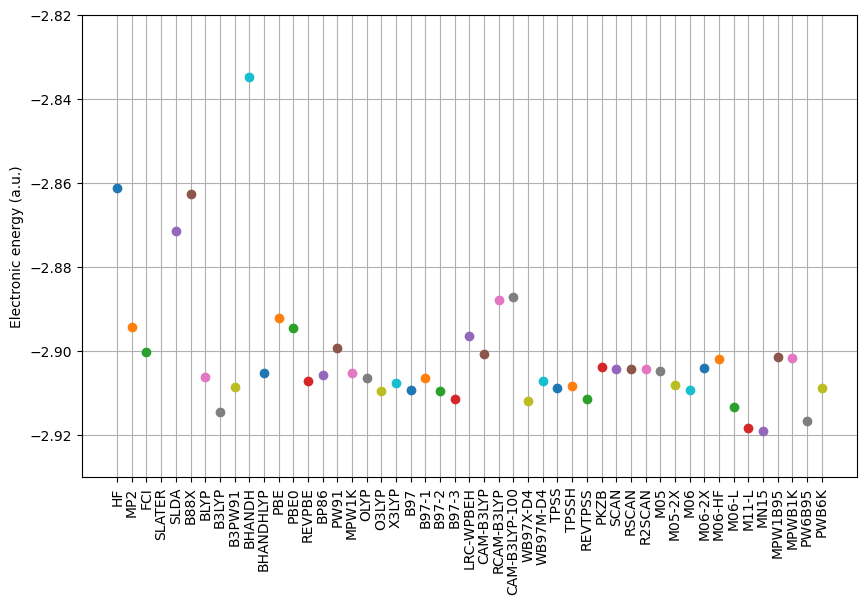
We will calculate the electronic energy of helium using the Hartree–Fock (HF), second-order Møller–Plesset (MP2), and full configuration interaction (FCI) methods as well as Kohn–Sham density functional theory (DFT) using the available XC functionals.

import matplotlib.pyplot as plt
import multipsi as mtp
import veloxchem as vlx

molecule = vlx.Molecule.read_molecule_string("He   0.000  0.000  0.000")
basis = vlx.MolecularBasis.read(molecule, "cc-pvtz", ostream=None)

Hartree–Fock¶

scf_drv = vlx.ScfRestrictedDriver()
scf_drv.ostream.mute()
scf_results = scf_drv.compute(molecule, basis)

energies = {}
energies["HF"] = scf_drv.get_scf_energy()

MP2¶

mp2_drv = vlx.Mp2Driver()
mp2_drv.ostream.mute()
mp2_results = mp2_drv.compute(molecule, basis, scf_drv.mol_orbs)

energies["MP2"] = mp2_results["mp2_energy"] + energies["HF"]

FCI¶

space = mtp.OrbSpace(molecule, scf_drv.mol_orbs)
space.fci()

ci_drv = mtp.CIDriver()
ci_drv.ostream.mute()

ci_results = ci_drv.compute(molecule, basis, space)

energies["FCI"] = ci_results["energies"][0]

DFT¶

for xcfun in vlx.available_functionals():
    scf_drv.xcfun = xcfun
    scf_drv.compute(molecule, basis)
    
    energies[xcfun] = scf_drv.get_scf_energy()

Plotting the energies¶

for method in energies.keys():
    print(f"    {method:<12s}: {energies[method]:16.8f} a.u.")

    HF          :      -2.86115334 a.u.
    MP2         :      -2.89429091 a.u.
    SLATER      :      -2.72271178 a.u.
    SLDA        :      -2.87143717 a.u.
    B88X        :      -2.86247050 a.u.
    BLYP        :      -2.90621759 a.u.
    B3LYP       :      -2.91450655 a.u.
    B3PW91      :      -2.90856296 a.u.
    BHANDH      :      -2.83473781 a.u.
    BHANDHLYP   :      -2.90514866 a.u.
    PBE         :      -2.89213590 a.u.
    PBE0        :      -2.89451563 a.u.
    REVPBE      :      -2.90710482 a.u.
    BP86        :      -2.90557480 a.u.
    PW91        :      -2.89919908 a.u.
    MPW1K       :      -2.90521521 a.u.
    OLYP        :      -2.90644600 a.u.
    O3LYP       :      -2.90951647 a.u.
    X3LYP       :      -2.90758515 a.u.
    B97         :      -2.90931588 a.u.
    B97-1       :      -2.90639481 a.u.
    B97-2       :      -2.90940855 a.u.
    B97-3       :      -2.91133188 a.u.
    LRC-WPBEH   :      -2.89632996 a.u.
    CAM-B3LYP   :      -2.90069339 a.u.
    RCAM-B3LYP  :      -2.88776421 a.u.
    CAM-B3LYP-100:      -2.88703797 a.u.
    WB97X-D4    :      -2.91197053 a.u.
    WB97M-D4    :      -2.90721813 a.u.
    TPSS        :      -2.90886838 a.u.
    TPSSH       :      -2.90836089 a.u.
    REVTPSS     :      -2.91132827 a.u.
    PKZB        :      -2.90387499 a.u.
    SCAN        :      -2.90431544 a.u.
    RSCAN       :      -2.90431544 a.u.
    R2SCAN      :      -2.90431544 a.u.
    M05         :      -2.90471113 a.u.
    M05-2X      :      -2.90804370 a.u.
    M06         :      -2.90925996 a.u.
    M06-2X      :      -2.90399052 a.u.
    M06-HF      :      -2.90187434 a.u.
    M06-L       :      -2.91319059 a.u.
    M11-L       :      -2.91833797 a.u.
    MPW1B95     :      -2.90141905 a.u.
    MPWB1K      :      -2.90163660 a.u.
    PW6B95      :      -2.91673962 a.u.
    PWB6K       :      -2.90888490 a.u.

fig, ax = plt.subplots(figsize=(10, 6))

for i, method in enumerate(energies.keys()):
    ax.plot(i, energies[method], "o")

ax.set_xticks(range(len(energies)), energies.keys())
plt.xticks(rotation=90)

ax.set_ylim(-2.93, -2.82)
plt.ylabel("Electronic energy (a.u.)")

plt.grid(True)
plt.show()