We will here go over the basics of using Jupyter notebooks with a focus on carrying out and analyzing quantum chemical calculations as well as different functions and routines that are used in eChem.
Cell types
A Jupyter notebook consists of a number of different cells which can be executed in any order, the most relevant being:
Markdown, where you write text and equations, insert hyperlinks, figures, and more
Code, which contains executable (Python) code
A cell is executed by marking the cell and pressing shift+enter, or the run botton at the top. For a markdown cell this formats the text, and for code cells it runs the code. You can also press ctrl+enter, which only runs the cell, while shift+enter runs the cell and then selects the next one. Results from cells are saved in memory, so it is often a good idea to separate complicated workflows into several blocks, e.g. performing heavy calculations in one block and doing post-processing in another block.
The cell-type is selected in a scroll-down window at the top of the notebook window, which for this cell is Markdown. For editing the formatted markdown cells you double-click on the text, which changes the format to plain text.
Markdown cells
Markdown is a lightweight language for creating formatted code, with syntax examples including:
# Heading 1

## Heading 2

### Heading 3

#### Heading 4
Results in headings of different levels, which are in a Jupyter book visible to the right.
You can write text
in **bold** or *italics*, and have

line breaks like this.
You can write text in bold or italics, and have
line breaks like this.
- Subject 1
    1. Detail 1
    2. Detail 2
- Subject 2
    - Another detail
1. New subject 1
Subject 1
Detail 1
Detail 2
Subject 2
Another detail
New subject 1
Can link to [wikipedia](https://www.wikipedia.org/).Can link to wikipedia.
Equations can be written with similar syntax as Latex, *e.g.*

$$
\overline{F} = m \overline{a}
$$

as well as in sentences, such as $\overline{F} = m \overline{a}$.
Equations can be written with similar syntax as Latex, e.g.
as well as in sentences, such as .
Markdown cells are used throughout eChem, and the above examples should cover the main functionalities you need to be familiar with. More examples can be found here.
Code cells
Code cells are written in Python, for which tutorials can be found, e.g., here and here.
As a basic example, we define a function in one cell (saving it in memory), and call this function in a different cell.
def sum_numbers(a, b):
    return a + b
sum_numbers(1, 2.0)3.0Assigning this to a variable and printing the results:
a = 1
b = 2.0
n_sum = sum_numbers(a, b)
print(n_sum)
3.0
Note that Python automatically assign variable type, and here understands that an integer and a float can be added together by converting the integer to a float.
We can print this with more advanced formatting, and add comments (#) in the code cells:
print(f"The sum of {a} and {b} is {n_sum}")

# tweaking position, number of decimals, and notation format
print(f"The sum of {a:2d} and {b:5.4f} is {n_sum:.2E}")
The sum of 1 and 2.0 is 3.0
The sum of 1 and 2.0000 is 3.00E+00
If you have the jupyterlab_code_formatter package installed (included in the eChem environment), you can format the code cells by running the Format notebook command at the top of the window (between cell type selection and the clock symbol). This will, for instance, take the following code cell:
import numpy as np
import matplotlib.pyplot as plt


import veloxchem as vlx
call_funtion(argument1, argument2,argument3,   argument4,argument5) # commenting this function
And reformat this to a to:
import matplotlib.pyplot as plt
import numpy as np
import veloxchem as vlx

call_funtion(
    argument1, argument2, argument3, argument4, argument5
)  # commenting this function
Python ecosystem
One of the advantages of Python is the extensive number of available modules and packages, with some examples including:
numpy: large collection of mathematical functionalitiesmatplotlib: library for plottingscipy: library for scientific and technical computingveloxchem: quantum chemical programpy3Dmol: for visualizing molecules
These modules can be loaded as a whole (often being given an alias to avoid function collisions and overwriting), or by loading specific functions. Loading the required modules for this notebook:
import matplotlib.pyplot as plt
import numpy as np
import py3Dmol as p3d
import scipy
import veloxchem as vlxFunctionalities from the packages are then used by calling the appropriate package and function, e.g. to print the value of we run:
print(np.pi)3.141592653589793
Molecular structure
Moving on to calculations of chemical systems, we consider water represented by the following xyz-string with atomic coordinates given in Ångström.
water_xyz = """3

O       0.0000000000     0.1178336003     0.0000000000
H      -0.7595754146    -0.4713344012    -0.0000000000
H       0.7595754146    -0.4713344012     0.0000000000
"""
Create a VeloxChem molecule object.
molecule = vlx.Molecule.read_xyz_string(water_xyz)Visualize
The molecule can be visualized using the show method. The resulting illustration that can be rotated and zoomed.
molecule.show()Electronic structure
The electronic structure of a molecule can be calculated using VeloxChem. A basis set needs to be specified.
basis = vlx.MolecularBasis.read(molecule, "6-31G", ostream=None)Details about the adopted basis set for this system can be obtained with the get_string method.
print(basis.get_string('Atomic Basis')) Molecular Basis (Atomic Basis)
================================
Basis: 6-31G
Atom Contracted GTOs Primitive GTOs
O (3S,2P) (10S,4P)
H (2S) (4S)
Contracted Basis Functions : 13
Primitive Basis Functions : 30
scf_drv = vlx.ScfRestrictedDriver()
scf_drv.ostream.mute()

scf_results = scf_drv.compute(molecule, basis)Results are stored in the scf_drv and scf_results objects and can be used for analysis, further calculations, and more. In order to better understand what an object is and what it contains, we can run:
scf_drv?Type: ScfRestrictedDriver
String form: <veloxchem.scfrestdriver.ScfRestrictedDriver object at 0x70a67e490e00>
File: ~/miniconda3/envs/echem/lib/python3.12/site-packages/veloxchem/scfrestdriver.py
Docstring:
Implements spin restricted closed shell SCF method with C2-DIIS and
two-level C2-DIIS convergence accelerators.
:param comm:
The MPI communicator.
:param ostream:
The output stream.
Init docstring:
Initializes spin restricted closed shell SCF driver to default setup
(convergence threshold, initial guess, etc) by calling base class
constructor.This returns the docstring and some basic information on the object. You can get more extensive information by running help(scf_drv):
help(scf_drv)Help on ScfRestrictedDriver in module veloxchem.scfrestdriver object:
class ScfRestrictedDriver(veloxchem.scfdriver.ScfDriver)
| ScfRestrictedDriver(comm=None, ostream=None)
|
| Implements spin restricted closed shell SCF method with C2-DIIS and
| two-level C2-DIIS convergence accelerators.
|
| :param comm:
| The MPI communicator.
| :param ostream:
| The output stream.
|
| Method resolution order:
| ScfRestrictedDriver
| veloxchem.scfdriver.ScfDriver
| builtins.object
|
| Methods defined here:
|
| __deepcopy__(self, memo)
| Implements deepcopy.
|
| :param memo:
| The memo dictionary for deepcopy.
|
| :return:
| A deepcopy of self.
|
| __init__(self, comm=None, ostream=None)
| Initializes spin restricted closed shell SCF driver to default setup
| (convergence threshold, initial guess, etc) by calling base class
| constructor.
|
| get_scf_type_str(self)
| Gets string for spin restricted closed shell SCF calculation.
| Overloaded base class method.
|
| :return:
| The string for spin restricted closed shell SCF calculation.
|
| ----------------------------------------------------------------------
| Methods inherited from veloxchem.scfdriver.ScfDriver:
|
| clear_start_orbitals(self)
| Clears the user-supplied start orbitals mode.
|
| compute(self, molecule, basis, min_basis=None)
| Performs SCF calculation using molecular data.
|
| :param molecule:
| The molecule.
| :param basis:
| The AO basis set.
| :param min_basis:
| The minimal AO basis set.
|
| compute_s2(self, molecule, ao_basis, scf_results)
| Computes expectation value of the S**2 operator.
|
| :param molecule:
| The molecule.
| :param ao_basis:
| The AO basis set.
| :param scf_results:
| The dictionary of tensors from converged SCF wavefunction.
|
| :return:
| Expectation value <S**2>.
|
| gen_initial_density_proj(self, molecule, ao_basis, valence_basis, valence_mo)
| Computes initial AO density from molecular orbitals obtained by
| inserting molecular orbitals from valence basis into molecular
| orbitals in full AO basis.
|
| :param molecule:
| The molecule.
| :param ao_basis:
| The AO basis.
| :param valence_basis:
| The valence AO basis for generation of molecular orbitals.
| :param valence_mo:
| The molecular orbitals in valence AO basis.
|
| :return:
| The AO density matrix.
|
| gen_initial_density_restart(self, molecule)
| Reads initial molecular orbitals and AO density from checkpoint file.
|
| :param molecule:
| The molecule.
|
| :return:
| The AO density matrix.
|
| gen_initial_density_sad(self, molecule, ao_basis, min_basis)
| Computes initial AO density using superposition of atomic densities
| scheme.
|
| :param molecule:
| The molecule.
| :param ao_basis:
| The AO basis.
| :param min_basis:
| The minimal AO basis for generation of atomic densities.
|
| :return:
| The AO density matrix.
|
| gen_initial_density_start_orbitals(self, molecule)
| Generates initial AO density from user-supplied orbitals.
|
| :param molecule:
| The molecule.
|
| :return:
| The AO density matrix.
|
| get_checkpoint_file(self)
| Gets the effective checkpoint file path.
|
| :return:
| The effective checkpoint file path, or None if unavailable.
|
| get_scf_energy(self)
| Gets SCF energy from previous SCF iteration.
|
| :return:
| The SCF energy.
|
| maximum_overlap(self, molecule, basis, orbitals, alpha_list, beta_list)
| Constraint the SCF calculation to find orbitals that maximize overlap
| with a reference set.
|
| :param molecule:
| The molecule.
| :param basis:
| The AO basis set.
| :param orbitals:
| The reference MolecularOrbital object.
| :param alpha_list:
| The list of alpha occupied orbitals.
| :param beta_list:
| The list of beta occupied orbitals.
|
| print_attributes(self)
| Prints attributes in SCF driver.
|
| print_keywords(self)
| Prints input keywords in SCF driver.
|
| read_settings(self, checkpoint_file)
| Reads SCF and method settings from checkpoint file.
|
| :param checkpoint_file:
| The checkpoint file to read settings from.
|
| set_start_orbitals(self, molecule, basis, array)
| Creates checkpoint file from numpy array containing starting orbitals.
|
| :param molecule:
| The molecule.
| :param basis:
| The AO basis set.
| :param array:
| The numpy array (or list/tuple of numpy arrays).
|
| update_settings(self, scf_dict, method_dict=None)
| Updates settings in SCF driver.
|
| :param scf_dict:
| The dictionary of scf input.
| :param method_dict:
| The dicitonary of method settings.
|
| validate_checkpoint(self, nuclear_charges, basis_set, scf_type)
| Validates the checkpoint file by checking nuclear charges and basis set.
|
| :param nuclear_charges:
| Numpy array of the nuclear charges.
| :param basis_set:
| Name of the AO basis.
| :param scf_type:
| The type of SCF calculation (restricted, unrestricted, or
| restricted_openshell).
|
| :return:
| Validity of the checkpoint file.
|
| write_checkpoint(self, molecule, basis)
| Writes molecular orbitals to checkpoint file.
|
| :param molecule:
| The molecule.
| :param basis:
| The AO basis set.
|
| ----------------------------------------------------------------------
| Readonly properties inherited from veloxchem.scfdriver.ScfDriver:
|
| comm
| Returns the MPI communicator.
|
| density
| Returns the density matrix.
|
| history
| Returns the SCF history.
|
| is_converged
| Returns whether SCF is converged.
|
| mol_orbs
| Returns the molecular orbitals (for backward compatibility).
|
| molecular_orbitals
| Returns the molecular orbitals.
|
| nnodes
| Returns the number of MPI processes.
|
| nodes
| Returns the number of MPI processes.
|
| num_iter
| Returns the current number of SCF iterations.
|
| ostream
| Returns the output stream.
|
| rank
| Returns the MPI rank.
|
| scf_energy
| Returns SCF energy.
|
| scf_results
| Returns the SCF results.
|
| scf_tensors
| Returns the SCF results.
|
| scf_type
| Returns the SCF type.
|
| ----------------------------------------------------------------------
| Data descriptors inherited from veloxchem.scfdriver.ScfDriver:
|
| __dict__
| dictionary for instance variables
|
| __weakref__
| list of weak references to the object
Finally, in order to see which instances and functions can be accessed, you can use auto-completion by writing scf_drv. and pressing tab. This shows all options with the same start as what you have written in a scroll-down window. For example, you can find a function called get_scf_energy, which returns the SCF energy:
print(scf_drv.get_scf_energy())-75.98387037576914
Visualize molecular orbitals
Molecular orbitals can be visualized using a light-weight, interactive function called OrbitalViewer. A viewer object is initiated, and provided information on the molecular structure, basis set, and SCF:
viewer = vlx.OrbitalViewer()
viewer.plot(molecule, basis, scf_drv.mol_orbs)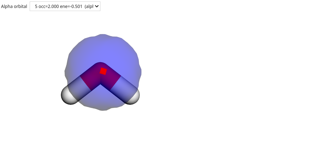
This results in seven molecular orbitals (selected by drop-down menu at the lower left), as the use of a minimal basis set (STO-3G) yields one basis function per hydrogen (1s), and five basis functions for oxygen (1s, 2s, and three 2p). You can change the visualization options in the upper right menu, with, e.g., the selected isosurface values under Objects>Orbitals>... (positive/negative isosurfaces are treated individually).
Basis set effects
Next, let us consider impact of different basis sets on the total energy, and see if there are any general trends for increasing basis set sizes. First, define a function which takes a molecular structure and basis set, and return the SCF energy and number of basis functions:
def calc_scf(xyz, basis):
    molecule = vlx.Molecule.read_xyz_string(xyz)
    basis = vlx.MolecularBasis.read(molecule, basis, ostream=None)
    n_bas = basis.get_dimensions_of_basis()
    scf_drv = vlx.ScfRestrictedDriver()
    scf_drv.ostream.mute()
    scf_results = scf_drv.compute(molecule, basis)
    scf_energy = scf_drv.get_scf_energy()
    return scf_energy, n_bas
Python lists
Create two empty lists for storing SCF energies and basis set sizes:
scf_energies = []
basis_size = []
Python lists are collections of elements (numbers, strings, other lists, ...), which can be modified. A list can be created by placing these elements within brackets, e.g:
list_example = [0.0, "Cat", np.pi, ["dog", np.e]]The individual elements can be called:
print(list_example[0])
print(list_example[1] + " and " + list_example[3][0])
0.0
Cat and dog
Or using a for loop:
for example in list_example:
    print(example)
0.0
Cat
3.141592653589793
['dog', 2.718281828459045]
Next, calculate the SCF energies and basis set sizes when using the following basis sets:
STO-3G
6-31G
6-311G
6-31++G**
6-311++G**
Details on what the basis set designations mean can be found elsewhere, e.g. here or in wikipedia. Create a list of basis set strings and run calc_scf:
basis_sets = ["STO-3G", "6-31G", "6-311G", "6-31++G**", "6-311++G**"]
for basis_set in basis_sets:
    energy_tmp, n_bas_tmp = calc_scf(water_xyz, basis_set)
    scf_energies.append(energy_tmp)
basis_size.append(n_bas_tmp)Plotting results
Next, construct a basic figure by initiating a figure object, plot the basis set size and SCF energy, and show the results:
plt.figure()
plt.plot(basis_size, scf_energies)
plt.show()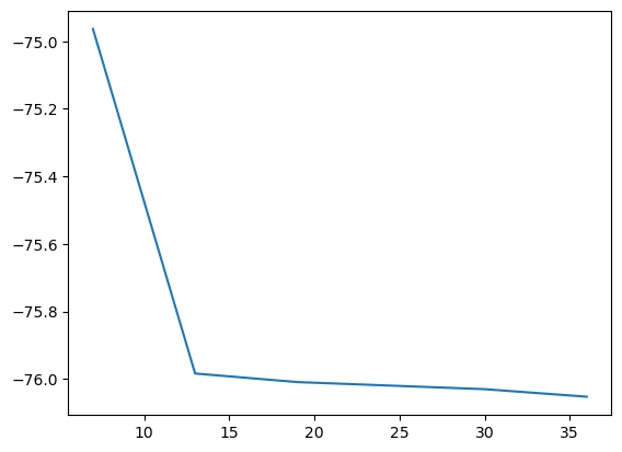
Tweaking the plot setting for a more appealing figure:
plt.figure(figsize=(5, 3.5)) # Tweak figure size
plt.title("Nicer figure") # Title

# plot circles at points, connected with a dashed line:
plt.plot(basis_size, scf_energies, "d--", color='red', label="Line")

plt.legend() # insert legend, using defined label
plt.xlim((6.0, 37.0)) # limits of x-axis
plt.ylim((-76.2, -74.8)) # limits of y-axis
plt.grid() # Include a grid
plt.xlabel("Basis set size")
plt.ylabel("Total energy [Hartree]")
plt.show()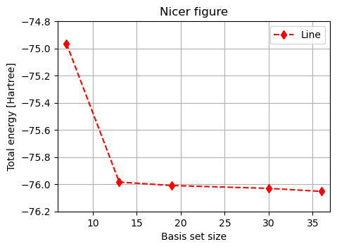
It is clear that the total energy decrease with basis set size, as a larger basis set generally provide more flexibility. This is not always the case, as smaller basis sets can be more suitable for describing a particular electronic structure.
Potential energy surfaces
An important concept in computational chemistry is that of the potential energy surface (PES), which describe the energy of a system as a function of some parameter (typically atomic positions). We here wish to construct this for carbon monoxide, by tracking the total energy as a function of the bond length.
Constructing a PES
In order to create a list of bond distances we can use np.arange or np.linspace, which returns evenly spaced values within a given interval. These values are returned using either a specified step length (np.arange), or a specified number of steps (np.linspace). Note that np.arange gives values up to, but not including, the end point.
print("np.arange:")
print(np.arange(10.0))
print(np.arange(start=1.0, stop=10.0, step=2.0))
print()
print("np.linspace:")
print(np.linspace(0.0, 10.0, 3))
print(np.linspace(start=1.0, stop=10.0, num=6))
np.arange:
[0. 1. 2. 3. 4. 5. 6. 7. 8. 9.]
[1. 3. 5. 7. 9.]
np.linspace:
[ 0. 5. 10.]
[ 1. 2.8 4.6 6.4 8.2 10. ]
We write 10.0 instead of 10 to ensure that Python understand that we want float numbers.
For calculating the PES we will use the replace command, which works as follows:
start_str = "John went bowling with Jane."
print(start_str)

end_str = start_str.replace("John", "Andrew")
end_str = end_str.replace("bowling", "to the cinema")
end_str = end_str.replace("Jane", "Sarah")
print(end_str)
John went bowling with Jane.
Andrew went to the cinema with Sarah.
Next, we use np.arange, replace, and calc_scf to create the PES.
co_base = """2

O       0.0       0.0       0.0
C         L       0.0       0.0
"""

bond_e = []
bond_l = np.arange(1.00, 1.40, 0.04)

for l in bond_l:
    co_tmp = co_base.replace("L", "{}".format(l))  # change C position
    energy_tmp, n_bas_tmp = calc_scf(co_tmp, "STO-3G")
    bond_e.append(energy_tmp)
Plot the resulting PES:
plt.figure(figsize=(5, 3.5))
plt.plot(bond_l, bond_e, "o-")
plt.show()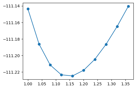
Interpolation with spline
A smoother, more aesthetically pleasing figure line can be constructed by using spline, which interpolate between data points with piece-wise polynomials of a desired order. A cubic spline tends to yield relatively smooth curves, and can be constructed as:
plt.figure(figsize=(5, 3.5))
plt.plot(bond_l, bond_e, "o")
spline_func = scipy.interpolate.interp1d(bond_l, bond_e, kind="cubic")
x_spline = np.linspace(min(bond_l), max(bond_l), 100)
y_spline = spline_func(x_spline)
plt.plot(x_spline, y_spline)
plt.legend(("Data", "Cubic spline"))
plt.show()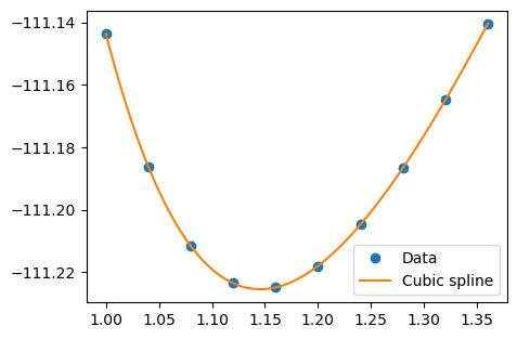
Fit harmonic function
The change in energy by bond stretch can be approximated as a harmonic potential:
Such potential fits can be used to form a force field which are then used for molecular dynamics. In order to do this, we will use scipy.optimize.curve_fit for optimizing the parameters. For this, we shift the energy so that the minima is zero and define the function to be fitted:
bond_e_shifted = np.array(bond_e) - min(bond_e)


def harmonic_func(l, l_0, k_s):
    return (k_s / 2.0) * (l - l_0) ** 2
Optimize the parameters and plot the results:
popt, pcov = scipy.optimize.curve_fit(harmonic_func, bond_l, bond_e_shifted)

plt.figure(figsize=(5, 3.5))
plt.plot(bond_l, bond_e_shifted, "d")
l = np.linspace(min(bond_l), max(bond_l), 100)
plt.plot(l, harmonic_func(l, *popt))
plt.show()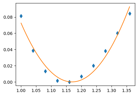
This fit takes the approximate shape of the calculate PES, but with a minima in the wrong location and an incorrect shape. This is due to a number of factor, including the inadequacies of a harmonic potential and fitting it to a somewhat unsuitable region, as discussed more here.
Functions and examples
Einstein summation
This e-book and our software makes use of np.einsum as a simple tool for performing Einstein summation, which is descried in the manual, and with basic examples found here.
Consider a vector A and a matrix B:
A = np.array([0, 1, 2])
B = np.array([[1, 1, 3], [3, 4, 5], [5, 6, 7]])

print("A:\n", A)
print("\nB:\n", B)
# \n adds a new line
A:
[0 1 2]
B:
[[1 1 3]
[3 4 5]
[5 6 7]]
print(np.einsum("i,ij->i", A, B))[ 0 12 36]
Here and select axis in the objects, and you can change the indices to any letter (provided you use them consistently). The operation carried out takes all and multiply with , summing over and returning a new object with elements along . Removing the on the right-hand side instead gives the total sum:
print(np.einsum("i,ij->", A, B))48
In other words, repeating an index tells np.einsum that it should multiply the objects along these dimensions, and omitting on the right-hand side tells it to sum along that dimension.
This can be used for simpler operations such as taking the sum of an object, performing element-wise multiplication, calculating the trace, and more. It can also be used for more complicated matrix-matrix operations and considering more arrays, and we will use it to perform a transformation from atomic to molecular orbitals (AO and MO, respectively).
AO to MO transformation
Integrals are calculate in an atomic orbital (AO) basis, while we would in most cases prefer to work in the molecular orbital (MO) basis. For this, we then need to perform an AO to MO transformation. As an example, consider the expectation value of the kinetic energy:
First, calculate the SCF of water with a minimal basis:
molecule = vlx.Molecule.read_xyz_string(water_xyz)
basis = vlx.MolecularBasis.read(molecule, "STO-3G")
From VeloxChem we have access to in the AO basis:
T_ao = vlx.compute_kinetic_energy_integrals(molecule, basis)Run the SCF to get the number of occupied orbitals and MO coefficient matrix:
scf_drv = vlx.ScfRestrictedDriver()
scf_drv.ostream.mute()
scf_results = scf_drv.compute(molecule, basis)

nocc = molecule.number_of_alpha_electrons()
C = scf_results["C_alpha"]
We calculate the elements of the kinetic energy operator from the transformation:
The MO coefficient matrix is real, so you can here ignore the complex conjugate.
We will use np.einsum to construct , and use the results to calculate the expectation value of the kinetic energy operator from before. For we need to know how to slice NumPy arrays.
As an example, the orbital energies are extracted as:
orbital_energies = scf_results["E_alpha"]
print(orbital_energies)
[-20.24238976 -1.26646064 -0.61558541 -0.45278477 -0.39106557
0.60181633 0.73720765]
To print the energy of the occupied and unoccupied orbitals we use splicing:
print("Energy of occupied:\n", orbital_energies[:nocc])
print("Energy of unoccupied:\n", orbital_energies[nocc:])
Energy of occupied:
[-20.24238976 -1.26646064 -0.61558541 -0.45278477 -0.39106557]
Energy of unoccupied:
[0.60181633 0.73720765]
When using np.einsum, look at the above equation and use this to guide the construction of the operation, following the same order of indices and variable (but interchanging the left- and right-hand sides). The order is on the left-hand side, and , , and on the right-hand side, so the summation becomes:
T_mo = np.einsum("ap, bq, ab -> pq", C, C, T_ao)Finally, the expectation value of the kinetic operator is:
T_exp = 2 * np.einsum("ii", T_mo[:nocc, :nocc])
print(f"Expectation value: {T_exp:.3f} Hartree")
Expectation value: 74.579 Hartree
Eigenvalues and eigenvectors
The eigenvalues and eigenvectors of a Hermitian matrix can be calculated with np.linalg.eigh(), and as an example we consider the overlap matrix (). This is constructed from the overlap between each pair of orbitals:
The overlap matrix is available as:
S = scf_results["S"]
print(np.around(S, 3))  # Rounding to three decimals
[[ 1. 0.237 0.053 0.053 0. 0. 0. ]
[ 0.237 1. 0.472 0.472 0. 0. 0. ]
[ 0.053 0.472 1. 0.25 -0.24 0. -0.31 ]
[ 0.053 0.472 0.25 1. -0.24 0. 0.31 ]
[ 0. 0. -0.24 -0.24 1. 0. 0. ]
[ 0. 0. 0. 0. 0. 1. 0. ]
[ 0. 0. -0.31 0.31 0. 0. 1. ]]
When constructing an orthogonal AO basis (see here) we diagonalize the overlap matrix:
collects the eigenvectors of as columns, which can be found using np.linalg.eigh:
s, U = np.linalg.eigh(S)

print("Eigenvalues:\n", np.around(s, 3))
print()  # print empty line
print("Eigenvectors:\n", np.around(U, 3))
Eigenvalues:
[0.345 0.42 0.886 1. 1.093 1.331 1.926]
Eigenvectors:
[[ 0.18 -0. -0.713 0. 0.644 0. -0.209]
[-0.695 -0. 0.279 0. 0.313 0. -0.584]
[ 0.437 -0.564 0.145 0. -0.131 -0.426 -0.52 ]
[ 0.437 0.564 0.145 0. -0.131 0.426 -0.52 ]
[ 0.321 -0. 0.609 0. 0.673 0. 0.27 ]
[ 0. 0. 0. 1. 0. 0. 0. ]
[-0. -0.602 -0. 0. -0. 0.798 -0. ]]
can be constructed using the eigenvectors and np.matmul:
S_diag = np.matmul(np.matmul(U.T, S), U)

print(np.around(S_diag, 3))
[[ 0.345 0. 0. 0. 0. 0. 0. ]
[ 0. 0.42 0. 0. -0. -0. -0. ]
[-0. 0. 0.886 0. 0. -0. 0. ]
[ 0. 0. 0. 1. 0. 0. 0. ]
[ 0. -0. 0. 0. 1.093 -0. 0. ]
[ 0. -0. -0. 0. -0. 1.331 0. ]
[ 0. -0. 0. 0. 0. 0. 1.926]]
Next, verify that :
print(np.around(np.matmul(U.T, U), 5))[[ 1. 0. 0. 0. 0. 0. 0.]
[ 0. 1. 0. 0. 0. 0. -0.]
[ 0. 0. 1. 0. 0. -0. 0.]
[ 0. 0. 0. 1. 0. 0. 0.]
[ 0. 0. 0. 0. 1. -0. 0.]
[ 0. 0. -0. 0. -0. 1. 0.]
[ 0. -0. 0. 0. 0. 0. 1.]]
Next, we can construct the diagonal matrix using the eigenvalues in and verify that it gives the same results as above.
For an identity matrix of dimension n we use np.identity(n).
print(np.around(s * np.identity(len(s)), 3))
print()
abs_diff = np.abs(s * np.identity(len(s)) - S_diag)
print(f"Summed absolute difference: {np.sum(abs_diff): .4E}")
[[0.345 0. 0. 0. 0. 0. 0. ]
[0. 0.42 0. 0. 0. 0. 0. ]
[0. 0. 0.886 0. 0. 0. 0. ]
[0. 0. 0. 1. 0. 0. 0. ]
[0. 0. 0. 0. 1.093 0. 0. ]
[0. 0. 0. 0. 0. 1.331 0. ]
[0. 0. 0. 0. 0. 0. 1.926]]
Summed absolute difference: 7.0866E-15
Dictionaries
Dictionaries are ordered collections of items, arranges in pairs of key and value:
some_dict = {"fruit": "apple", "color": "red"}

print("Print keys:")
print(some_dict.keys())

print("\nPrint values:")
print(some_dict.values())

print("\nPrint specific value:")
print(some_dict["color"])
Print keys:
dict_keys(['fruit', 'color'])
Print values:
dict_values(['apple', 'red'])
Print specific value:
red
You can change values and add more keys:
some_dict["color"] = "green"
print(some_dict.values())
print()
some_dict["freshness"] = "ripe"
print(some_dict.keys())
print()
print(some_dict.values())
dict_values(['apple', 'green'])
dict_keys(['fruit', 'color', 'freshness'])
dict_values(['apple', 'green', 'ripe'])
The elements of a dictionary can be another dictionary:
some_dict["dimensions"] = {"length": 4.5, "width": 4.3, "height": 5.2}
print(some_dict.values())
dict_values(['apple', 'green', 'ripe', {'length': 4.5, 'width': 4.3, 'height': 5.2}])
x = some_dict["dimensions"]
print(x)
print()
print(x.keys())
print()
print(x["width"])
{'length': 4.5, 'width': 4.3, 'height': 5.2}
dict_keys(['length', 'width', 'height'])
4.3
Function isinstance
This function checks if an object is of the specified type:
x = 5
print("Is x a string:  ", isinstance(x, str))
print("Is x an integer:", isinstance(x, int))
print("Is x a float:   ", isinstance(x, float))
Is x a string: False
Is x an integer: True
Is x a float: False
Functions np.zeros and np.ones
These functions return object of certain dimension, composed of zeros or ones.
print(np.zeros((3, 2)))
print(np.ones((6)))
[[0. 0.]
[0. 0.]
[0. 0.]]
[1. 1. 1. 1. 1. 1.]
Functions np.rad2deg and np.deg2rad
Convert angles between radians (which are the default in Python) and degrees.
print(f"{np.rad2deg(np.pi/4.):.2f}")
print(f"{np.deg2rad(45.):.3f}")
45.00
0.785
External websites and tutorials
We have chosen to use Python as the high-level programming and interfacing layer on account of its flexibility, ease of use, and extensive ecosystem. As the framework for carrying out the calculation and analysis, as well as enabling the intermingling of calculation and text, we use Jupyter. If you are unfamiliar in the use of these software packages, there is a wealth of resources which can help you get better accomodated with these tools, such as:
For Python you can start with W3Schools, which hosts comprehensive tutorials for a large number of programming languages and modules, or the tutorial from the Python project.
For Jupyter you can find examples or test on the project page, prepared lessons, and video tutorials.
The construction of Jupyter books is documented on the host site, which also contains a gallery of different e-books, such as this one dedicated to teaching scientific computing for chemists (describing the use Python, Jupyter, and more), or this page.
The use of JupyterHub for serving Jupyter notebooks for multiple users is described on the project page, with instructions on how to deploy it on a cloud found here.
For visualization there are examples and tutorials for using
matplotlibon the project page and W3Schools, and you can also look at tutorials for the high-level seaborn visualization library.