Full-CI response
As we saw in the previous section, for an exact state, we have the formula
For example, in the case of a molecule irradiated by light, we are interested in computing the polarizability , corresponding to the response with and , where . Looking more precisely at the isotropic component, , we obtain
We now define the oscillator strength for a transition as
such that
Those formulas can be applied directly for a configuration interaction wave function, where it is easy to get the excited state energies simply by obtaining additional roots in the diagonalization of the Hamiltonian. We then only need to compute the matrix element . In second quantization, the component of the dipole operator can be written as
We thus need to compute the matrix , with elements , which is called the transition density matrix, and contract it with the dipole moment integrals.
Let’s apply these for full CI (FCI) of a water molecule.
import veloxchem as vlx
import multipsi as mtp
import numpy as np
mol_str = """3
O 0.0000000000 0.0000000000 0.1178336003
H -0.7595754146 -0.0000000000 -0.4713344012
H 0.7595754146 0.0000000000 -0.4713344012
"""
molecule = vlx.Molecule.read_xyz_string(mol_str)
basis = vlx.MolecularBasis.read(molecule, "6-31g")
scf_drv = vlx.ScfRestrictedDriver()
scf_results = scf_drv.compute(molecule, basis)# Compute the 5 lowest states of water using full CI
space=mtp.OrbSpace(molecule, basis, scf_drv.mol_orbs)
# Full CI with frozen 1s orbital
space.fci(n_frozen=1)
nstates=5
cidrv=mtp.CIDriver()
ci_results = cidrv.compute(molecule,basis,space,nstates)Output
                          Configuration Interaction Driver
                         ==================================


               Active space definition:
               ------------------------
               Number of inactive (occupied) orbitals: 1
               Number of active orbitals:              12
               Number of virtual orbitals:             0

               This is a CASSCF wavefunction: CAS(8,12)

               CI expansion:
               -------------
               Number of determinants:      245025


               ╭────────────────────────────────────╮
               │          Driver settings           │
               ╰────────────────────────────────────╯

               Max. iterations               :   40
               Initial diagonalization       :   205
               Convergence thresholds:
                - Energy change              :   1e-08
                - Residual square norm       :   1e-08
               Davidson solver
                - Max subspace size          :   50
                - Min subspace size          :   30
                - Standard Davidson step


                          CI Iterations
                         ----------------

     Iter. | Average Energy | E. Change | Grad. Norm | Subs. size | Time
     ----------------------------------------------------------------------
        1     -75.684672473    -4.3e-14      4.3e-01           5    0:00:00
        2     -75.788930816    -1.0e-01      5.1e-02          10    0:00:00
        3     -75.799112271    -1.0e-02      5.9e-03          15    0:00:00
        4     -75.800337767    -1.2e-03      1.0e-03          20    0:00:00
        5     -75.800533861    -2.0e-04      1.9e-04          25    0:00:00
        6     -75.800568191    -3.4e-05      3.8e-05          30    0:00:00
        7     -75.800573348    -5.2e-06      7.8e-06          35    0:00:00
        8     -75.800574691    -1.3e-06      5.4e-06          40    0:00:00
        9     -75.800575153    -4.6e-07      2.3e-06          45    0:00:00
       10     -75.800575306    -1.5e-07      5.7e-07          49    0:00:00
       11     -75.800575334    -2.8e-08      7.5e-08          30    0:00:00
       12     -75.800575338    -3.9e-09      1.5e-08          32    0:00:00
       13     -75.800575339    -8.5e-10      7.0e-09          33    0:00:00

** Convergence reached in 13 iterations

               Final results
               -------------

* State 1
  - S^2    : 0.00  (multiplicity = 1.0 )
  - Energy : -76.12020540259658
  - Natural orbitals
1.98825 1.96801 1.97145 1.98065 0.00050 0.02822 0.00310 0.01813 0.02666 0.01218 0.00063 0.00222

* State 2
  - S^2    : 0.00  (multiplicity = 1.0 )
  - Energy : -75.8096766321045
  - Natural orbitals
1.98999 1.96500 1.97826 0.99416 0.99612 0.03529 0.00360 0.00679 0.01598 0.00969 0.00250 0.00263

* State 3
  - S^2    : 0.00  (multiplicity = 1.0 )
  - Energy : -75.72755706076029
  - Natural orbitals
1.98934 1.97698 1.96858 0.99423 0.03496 0.99438 0.00381 0.00671 0.00220 0.01152 0.01394 0.00335

* State 4
  - S^2    : 0.00  (multiplicity = 1.0 )
  - Energy : -75.71682482310734
  - Natural orbitals
1.98622 1.95656 1.14202 1.98084 0.84833 0.04126 0.00283 0.01796 0.01163 0.00636 0.00360 0.00240

* State 5
  - S^2    : 0.00  (multiplicity = 1.0 )
  - Energy : -75.62861277525086
  - Natural orbitals
1.98447 1.95664 1.01095 1.98207 0.04114 0.97800 0.00370 0.01636 0.00441 0.00643 0.01380 0.00204
au2ev = 27.211386

# Get the molecular orbitals within the active space
C=space._get_active_mos()

# Compute dipole integrals in AO basis
dipole_drv = vlx.ElectricDipoleIntegralsDriver()
dipole_mats = dipole_drv.compute(molecule, basis)
dipole=[dipole_mats.x_to_numpy(),dipole_mats.y_to_numpy(),dipole_mats.z_to_numpy()]

# Transform to MO basis
dipole_mo=[]
for icomp in range(0,3):
    dipole_mo.append(np.einsum('pq,pt,qu->tu', dipole[icomp], C, C))


# Initialize the CIOperator class to compute the transition densities.
expansion=mtp.CIExpansion(space)
DenDriver=mtp.CIOperator(expansion, cidrv.comm)
energies = ci_results["energies"]
ci_vectors = ci_results["ci_vectors"]

# Compute all 0->n transitions
for n in range(1,nstates):
    dE=energies[n]-energies[0]
    tden=DenDriver.get_1dm(ci_vectors, 0, ci_vectors, n) #Transition density matrix
    dx=np.tensordot(tden, dipole_mo[0]) #<0|x|n>
    dy=np.tensordot(tden, dipole_mo[1]) #<0|y|n>
    dz=np.tensordot(tden, dipole_mo[2]) #<0|z|n>
    F=2/3*dE*(dx*dx+dy*dy+dz*dz)
    print(f"Excitation 0->{n} energy: {dE*au2ev:5.3f} eV oscillator strength: {F:.5f}")
Excitation 0->1 energy: 8.450 eV oscillator strength: 0.01319
Excitation 0->2 energy: 10.685 eV oscillator strength: 0.00000
Excitation 0->3 energy: 10.977 eV oscillator strength: 0.11536
Excitation 0->4 energy: 13.377 eV oscillator strength: 0.11503
We thus obtain 3 visible transitions and one dark state (near-zero dipole oscillator strength). We obtain the exact same result by using the built-in class of multipsi:
SI = mtp.StateInteraction()
si_results = SI.compute(molecule, basis, ci_results)
List of oscillator strengths greather than 1e-10

  From     to       Energy (eV)    Oscillator strength (length and velocity)
     1       2        8.44992         1.318942e-02    4.625244e-02
     1       4       10.97654         1.153567e-01    1.749731e-01
     1       5       13.37692         1.150314e-01    1.224456e-01

List of rotatory strengths greather than 1e-10

  From     to       Energy (eV)    Rot. strength (a.u. and 10^-40 cgs)
     1       2        8.44992         2.977592e-10    1.403767e-07
     1       5       13.37692        -3.389492e-09   -1.597954e-06
Truncated CI
In truncated CI, the energy does not just depend on the CI coefficients but also on the molecular orbitals, which makes the truncated CI response more complicated. However, it is interesting to look at the results we obtain by simply applying the above equations. This gives a hierarchy of method from CIS to full CI. However, the excitation energies do not necessarily improve from order to order. Let us demonstrate this on the water example.
nstates=5
# nstates-1 transitions for CIS, CISD, CISDT and CISDTQ and FCI
Energies=np.empty((5,nstates-1))
Energies[4,:]=au2ev*np.array(si_results['energies']) # Save the FCI result

#CIS to CISDTQ
space=mtp.OrbSpace(molecule, basis, scf_drv.mol_orbs)
cidrv=mtp.CIDriver()
SI=mtp.StateInteraction()

for exc in range(1,5):
    space.ci(exc,n_frozen=1)
    ci_results = cidrv.compute(molecule,basis,space, nstates)
    si_results = SI.compute(molecule,basis,ci_results)
    Energies[exc-1,:]=au2ev*np.array(si_results['energies'])
Output
                          Configuration Interaction Driver
                         ==================================


               Active space definition:
               ------------------------
               Number of inactive (occupied) orbitals: 1
               Number of active orbitals:              12
               Number of virtual orbitals:             0

               This is a GASSCF wavefunction

                        Cumulated   Min cumulated    Max cumulated
               Space     orbitals      occupation       occupation
                   1            4               7                8
                   2           12               8                8


               CI expansion:
               -------------
               Number of determinants:      65


               ╭────────────────────────────────────╮
               │          Driver settings           │
               ╰────────────────────────────────────╯

                Solved by explicit diagonalization


** Convergence reached in 0 iterations

               Final results
               -------------

* State 1
  - S^2    : 0.00  (multiplicity = 1.0 )
  - Energy : -75.98387037576907
  - Natural orbitals
2.00000 2.00000 2.00000 2.00000 -0.00000 -0.00000 0.00000 -0.00000 0.00000 0.00000 0.00000 0.00000

* State 2
  - S^2    : 0.00  (multiplicity = 1.0 )
  - Energy : -75.63914005464734
  - Natural orbitals
2.00000 2.00000 1.99997 1.00003 0.99997 -0.00000 0.00000 0.00003 0.00000 -0.00000 -0.00000 0.00000

* State 3
  - S^2    : -0.00  (multiplicity = 1.0 )
  - Energy : -75.5683315721095
  - Natural orbitals
2.00000 1.99997 2.00000 1.00003 -0.00000 0.99997 0.00000 0.00003 -0.00000 0.00000 0.00000 -0.00000

* State 4
  - S^2    : 0.00  (multiplicity = 1.0 )
  - Energy : -75.54906254741879
  - Natural orbitals
1.99959 1.98314 1.02031 1.99696 0.97969 0.01686 -0.00000 0.00304 0.00000 -0.00000 0.00000 0.00041

* State 5
  - S^2    : 0.00  (multiplicity = 1.0 )
  - Energy : -75.4729676559138
  - Natural orbitals
1.99995 1.97129 1.02876 2.00000 0.02871 0.97124 -0.00000 -0.00000 0.00000 0.00000 0.00005 0.00000

List of oscillator strengths greather than 1e-10

  From     to       Energy (eV)    Oscillator strength (length and velocity)
     1       2        9.38059         1.468873e-02    4.091187e-02
     1       4       11.83172         1.208787e-01    1.355740e-01
     1       5       13.90237         1.045445e-01    8.623011e-02

List of rotatory strengths greather than 1e-10

  From     to       Energy (eV)    Rot. strength (a.u. and 10^-40 cgs)

                          Configuration Interaction Driver
                         ==================================


               Active space definition:
               ------------------------
               Number of inactive (occupied) orbitals: 1
               Number of active orbitals:              12
               Number of virtual orbitals:             0

               This is a GASSCF wavefunction

                        Cumulated   Min cumulated    Max cumulated
               Space     orbitals      occupation       occupation
                   1            4               6                8
                   2           12               8                8


               CI expansion:
               -------------
               Number of determinants:      1425


               ╭────────────────────────────────────╮
               │          Driver settings           │
               ╰────────────────────────────────────╯

               Max. iterations               :   40
               Initial diagonalization       :   205
               Convergence thresholds:
                - Energy change              :   1e-08
                - Residual square norm       :   1e-08
               Davidson solver
                - Max subspace size          :   50
                - Min subspace size          :   30
                - Standard Davidson step


                          CI Iterations
                         ----------------

     Iter. | Average Energy | E. Change | Grad. Norm | Subs. size | Time
     ----------------------------------------------------------------------
        1     -75.684672473    -1.4e-14      4.3e-01           5    0:00:00
        2     -75.738323483    -5.4e-02      1.1e-02          10    0:00:00
        3     -75.740452179    -2.1e-03      4.8e-04          15    0:00:00
        4     -75.740697234    -2.5e-04      1.1e-04          20    0:00:00
        5     -75.740727930    -3.1e-05      1.4e-05          25    0:00:00
        6     -75.740732300    -4.4e-06      9.7e-06          30    0:00:00
        7     -75.740733488    -1.2e-06      1.3e-06          35    0:00:00
        8     -75.740733645    -1.6e-07      8.0e-08          40    0:00:00
        9     -75.740733654    -8.9e-09      6.9e-09          43    0:00:00
       10     -75.748719197    -8.0e-03      1.6e-01          44    0:00:00
       11     -75.764735822    -1.6e-02      5.8e-03          45    0:00:00
       12     -75.765384377    -6.5e-04      3.2e-04          48    0:00:00
       13     -75.765428572    -4.4e-05      4.0e-05          49    0:00:00
       14     -75.765434363    -5.8e-06      4.4e-06          50    0:00:00
       15     -75.765435179    -8.2e-07      7.0e-07          30    0:00:00
       16     -75.765435245    -6.6e-08      4.5e-08          31    0:00:00
       17     -75.765435250    -4.7e-09      2.2e-09          32    0:00:00
       18     -75.765435250    -2.6e-10      1.4e-10          33    0:00:00

** Convergence reached in 18 iterations

               Final results
               -------------

* State 1
  - S^2    : 0.00  (multiplicity = 1.0 )
  - Energy : -76.11340211624527
  - Natural orbitals
1.98980 1.97263 1.97571 1.98356 0.00034 0.02409 0.00268 0.01544 0.02279 0.01054 0.00046 0.00195

* State 2
  - S^2    : 0.00  (multiplicity = 1.0 )
  - Energy : -75.73519313668203
  - Natural orbitals
1.99830 1.99110 1.99600 0.99907 0.99382 0.01175 0.00118 0.00147 0.00444 0.00171 0.00035 0.00082

* State 3
  - S^2    : 2.00  (multiplicity = 3.0 )
  - Energy : -75.68094195702136
  - Natural orbitals
1.99572 1.98512 1.01018 1.99791 0.98621 0.01355 0.00151 0.00196 0.00508 0.00116 0.00063 0.00097

* State 4
  - S^2    : 0.00  (multiplicity = 1.0 )
  - Energy : -75.6540773260655
  - Natural orbitals
1.99830 1.99450 1.99144 0.99900 0.01390 0.99166 0.00117 0.00153 0.00080 0.00149 0.00575 0.00047

* State 5
  - S^2    : 0.00  (multiplicity = 1.0 )
  - Energy : -75.64356171394716
  - Natural orbitals
1.99571 1.97554 1.12840 1.99582 0.86456 0.02647 0.00142 0.00379 0.00507 0.00180 0.00051 0.00091

List of oscillator strengths greather than 1e-10

  From     to       Energy (eV)    Oscillator strength (length and velocity)
     1       2       10.29159         1.548860e-02    3.658372e-02
     1       5       12.78501         1.247443e-01    1.355467e-01

List of rotatory strengths greather than 1e-10

  From     to       Energy (eV)    Rot. strength (a.u. and 10^-40 cgs)

                          Configuration Interaction Driver
                         ==================================


               Active space definition:
               ------------------------
               Number of inactive (occupied) orbitals: 1
               Number of active orbitals:              12
               Number of virtual orbitals:             0

               This is a GASSCF wavefunction

                        Cumulated   Min cumulated    Max cumulated
               Space     orbitals      occupation       occupation
                   1            4               5                8
                   2           12               8                8


               CI expansion:
               -------------
               Number of determinants:      12625


               ╭────────────────────────────────────╮
               │          Driver settings           │
               ╰────────────────────────────────────╯

               Max. iterations               :   40
               Initial diagonalization       :   205
               Convergence thresholds:
                - Energy change              :   1e-08
                - Residual square norm       :   1e-08
               Davidson solver
                - Max subspace size          :   50
                - Min subspace size          :   30
                - Standard Davidson step


                          CI Iterations
                         ----------------

     Iter. | Average Energy | E. Change | Grad. Norm | Subs. size | Time
     ----------------------------------------------------------------------
        1     -75.684672473     0.0e+00      4.3e-01           5    0:00:00
        2     -75.784612942    -1.0e-01      2.0e-02          10    0:00:00
        3     -75.791286693    -6.7e-03      2.6e-03          15    0:00:00
        4     -75.792084611    -8.0e-04      3.8e-04          20    0:00:00
        5     -75.792189647    -1.1e-04      4.8e-05          25    0:00:00
        6     -75.792203247    -1.4e-05      2.0e-05          30    0:00:00
        7     -75.792206264    -3.0e-06      6.6e-06          35    0:00:00
        8     -75.792207573    -1.3e-06      4.0e-06          40    0:00:00
        9     -75.792207901    -3.3e-07      5.1e-07          44    0:00:00
       10     -75.792207946    -4.4e-08      5.5e-08          47    0:00:00
       11     -75.792207950    -4.4e-09      6.2e-09          49    0:00:00
       12     -75.792207951    -4.5e-10      2.6e-09          50    0:00:00

** Convergence reached in 12 iterations

               Final results
               -------------

* State 1
  - S^2    : 0.00  (multiplicity = 1.0 )
  - Energy : -76.11438963615075
  - Natural orbitals
1.98960 1.97168 1.97493 1.98327 0.00047 0.02478 0.00289 0.01562 0.02338 0.01071 0.00060 0.00208

* State 2
  - S^2    : 0.00  (multiplicity = 1.0 )
  - Energy : -75.80003060638765
  - Natural orbitals
1.99159 1.97001 1.98187 0.99537 0.99592 0.03029 0.00318 0.00554 0.01330 0.00820 0.00236 0.00237

* State 3
  - S^2    : 0.00  (multiplicity = 1.0 )
  - Energy : -75.71893849611735
  - Natural orbitals
1.99111 1.97998 1.97319 0.99537 0.03033 0.99427 0.00339 0.00552 0.00197 0.00953 0.01223 0.00311

* State 4
  - S^2    : 0.00  (multiplicity = 1.0 )
  - Energy : -75.70731803920357
  - Natural orbitals
1.98804 1.96044 1.12926 1.98430 0.86217 0.03726 0.00263 0.01467 0.01016 0.00542 0.00348 0.00217

* State 5
  - S^2    : 0.00  (multiplicity = 1.0 )
  - Energy : -75.62036297595392
  - Natural orbitals
1.98665 1.95754 1.01384 1.98540 0.04013 0.97606 0.00341 0.01331 0.00417 0.00547 0.01214 0.00187

List of oscillator strengths greather than 1e-10

  From     to       Energy (eV)    Oscillator strength (length and velocity)
     1       2        8.55414         1.328929e-02    4.580098e-02
     1       4       11.07698         1.154310e-01    1.705735e-01
     1       5       13.44315         1.119829e-01    1.181224e-01

List of rotatory strengths greather than 1e-10

  From     to       Energy (eV)    Rot. strength (a.u. and 10^-40 cgs)

                          Configuration Interaction Driver
                         ==================================


               Active space definition:
               ------------------------
               Number of inactive (occupied) orbitals: 1
               Number of active orbitals:              12
               Number of virtual orbitals:             0

               This is a GASSCF wavefunction

                        Cumulated   Min cumulated    Max cumulated
               Space     orbitals      occupation       occupation
                   1            4               4                8
                   2           12               8                8


               CI expansion:
               -------------
               Number of determinants:      55325


               ╭────────────────────────────────────╮
               │          Driver settings           │
               ╰────────────────────────────────────╯

               Max. iterations               :   40
               Initial diagonalization       :   205
               Convergence thresholds:
                - Energy change              :   1e-08
                - Residual square norm       :   1e-08
               Davidson solver
                - Max subspace size          :   50
                - Min subspace size          :   30
                - Standard Davidson step


                          CI Iterations
                         ----------------

     Iter. | Average Energy | E. Change | Grad. Norm | Subs. size | Time
     ----------------------------------------------------------------------
        1     -75.684672473    -5.7e-14      4.3e-01           5    0:00:00
        2     -75.788930816    -1.0e-01      4.8e-02          10    0:00:00
        3     -75.798239112    -9.3e-03      3.9e-03          15    0:00:00
        4     -75.799234656    -1.0e-03      7.9e-04          20    0:00:00
        5     -75.799415298    -1.8e-04      1.3e-04          25    0:00:00
        6     -75.799440760    -2.5e-05      2.3e-05          30    0:00:00
        7     -75.799445003    -4.2e-06      5.0e-06          35    0:00:00
        8     -75.799446153    -1.1e-06      4.4e-06          40    0:00:00
        9     -75.799446589    -4.4e-07      1.6e-06          45    0:00:00
       10     -75.799446717    -1.3e-07      2.5e-07          49    0:00:00
       11     -75.799446735    -1.8e-08      3.9e-08          30    0:00:00
       12     -75.799446738    -2.4e-09      6.0e-09          31    0:00:00
       13     -75.799446738    -4.1e-10      4.5e-09          32    0:00:00

** Convergence reached in 13 iterations

               Final results
               -------------

* State 1
  - S^2    : 0.00  (multiplicity = 1.0 )
  - Energy : -76.12003281944091
  - Natural orbitals
1.98832 1.96820 1.97163 1.98078 0.00049 0.02805 0.00308 0.01801 0.02650 0.01210 0.00062 0.00221

* State 2
  - S^2    : 0.00  (multiplicity = 1.0 )
  - Energy : -75.80828932705683
  - Natural orbitals
1.99041 1.96630 1.97922 0.99448 0.99598 0.03407 0.00351 0.00646 0.01523 0.00935 0.00243 0.00257

* State 3
  - S^2    : 0.00  (multiplicity = 1.0 )
  - Energy : -75.72622989915607
  - Natural orbitals
1.98982 1.97785 1.96970 0.99453 0.03391 0.99421 0.00372 0.00639 0.00215 0.01098 0.01350 0.00324

* State 4
  - S^2    : 0.00  (multiplicity = 1.0 )
  - Energy : -75.71537749183258
  - Natural orbitals
1.98672 1.95763 1.14166 1.98172 0.84887 0.04031 0.00280 0.01710 0.01128 0.00608 0.00347 0.00235

* State 5
  - S^2    : 0.00  (multiplicity = 1.0 )
  - Energy : -75.62730415289583
  - Natural orbitals
1.98504 1.95736 1.01139 1.98291 0.04057 0.97776 0.00364 0.01556 0.00426 0.00615 0.01336 0.00200

List of oscillator strengths greather than 1e-10

  From     to       Energy (eV)    Oscillator strength (length and velocity)
     1       2        8.48297         1.323128e-02    4.607677e-02
     1       4       11.01123         1.154582e-01    1.737606e-01
     1       5       13.40783         1.150823e-01    1.218343e-01

List of rotatory strengths greather than 1e-10

  From     to       Energy (eV)    Rot. strength (a.u. and 10^-40 cgs)
     1       2        8.48297         2.290063e-13    1.079635e-10
     1       5       13.40783         5.992948e-11    2.825337e-08
        6     -75.799446125    -9.5e-06      3.3e-06   0:00:08
        7     -75.799446623    -9.0e-07      5.5e-07   0:00:08
        8     -75.799446711    -2.5e-07      2.1e-07   0:00:08
        9     -75.799446734    -9.2e-08      6.1e-08   0:00:07
       10     -75.799446738    -2.0e-08      7.4e-09   0:00:07
       11     -75.799446739    -2.1e-09      8.5e-10   0:00:10

** Convergence reached in 11 iterations

        Final results
        -------------


* State 1
- Energy: -76.12003281964515
- S^2   : -0.02  (multiplicity = 1.0 )
- Natural orbitals
1.98832 1.96820 1.97163 1.98078 0.00049 0.02805 0.00308 0.01801 0.02650 0.01210 0.00062 0.00221

* State 2
- Energy: -75.80828932732831
- S^2   : -0.03  (multiplicity = 0.9 )
- Natural orbitals
1.99041 1.96630 1.97922 0.99448 0.99598 0.03407 0.00351 0.00646 0.01523 0.00935 0.00243 0.00257

* State 3
- Energy: -75.72622990160053
- S^2   : -0.03  (multiplicity = 0.9 )
- Natural orbitals
1.98982 1.97785 1.96971 0.99453 0.03391 0.99421 0.00372 0.00639 0.00215 0.01098 0.01350 0.00324

* State 4
- Energy: -75.71537749268845
- S^2   : -0.03  (multiplicity = 0.9 )
- Natural orbitals
1.98672 1.95763 1.14165 1.98172 0.84888 0.04031 0.00280 0.01710 0.01128 0.00608 0.00347 0.00235

* State 5
- Energy: -75.6273041535162
- S^2   : -0.03  (multiplicity = 0.9 )
- Natural orbitals
1.98504 1.95735 1.01140 1.98291 0.04058 0.97774 0.00364 0.01556 0.00427 0.00615 0.01336 0.00427

List of oscillator strengths greather than 1e-10

  From     to       Energy (eV)    Oscillator strength (length and velocity)
     1       2        8.48297         1.323123e-02    4.607713e-02
     1       4       11.01123         1.154562e-01    1.737591e-01
     1       5       13.40783         1.150580e-01    1.218071e-01

List of rotatory strengths greater than 1e-10

  From     to       Energy (eV)    Rot. strength (a.u. and 10^-40 cgs)
import matplotlib.pyplot as plt

plt.figure(figsize=(6,4))
x = np.array(range(1,6))
plt.plot(x,Energies[:,0], label='0->1')
plt.plot(x,Energies[:,1], label='0->2')
plt.plot(x,Energies[:,2], label='0->3')
plt.plot(x,Energies[:,3], label='0->4')

plt.title('Convergence of excitation energies')
plt.xticks([1, 2, 3, 4, 5], ['CIS', 'CISD', 'CISDT', 'CISDTQ', 'FCI'])
plt.ylabel("Energies (eV)")
plt.legend()
plt.tight_layout(); plt.show()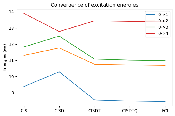
Energies[0,:]array([ 9.38058983, 11.30738678, 11.83172365, 13.90237112])As we can see, we do not have a monotonous convergence towards the full CI result. In particular, CISD is actually worse than CIS. The reason for this is that CIS has a more even-handed treatment of the ground and excited states than CISD. In CIS, due to the Brillouin theorem, the ground state does not improve with the inclusion of single excitations, but the single excitations are needed to generate the dominant configuration for the (singly) excited states. Both ground and excited states are thus treated at a mean-field (HF-like) level.
However, in CISD, the ground state contains double excitation, and thus dynamical correlation, while the excited states would need up to triple excitations to both generate the singly-excited dominant configuration and correlating double excitations on top. There is an unbalance, the ground state being described more accurately than the excited states, leading to too high excitation energies. Adding the triple excitations bring correlation also for excited states, which brings the result closer to the final FCI result, and in this simple case is essentially converged.
For this reason, while CIS is sometimes used to compute excitation energies (and as we can see in the next section, is actually related to HF response), the other truncated CIs are not.