Natural transition orbitals

Natural transitions orbitals (NTOs) are designed to provide a compact representation of the transition density matrix Martin (2003).

If we collect occupied and unoccupied (real) MOs as row and column vectors, repsectively,

\bar{\phi}_\mathrm{occ}(\mathbf{r}) = (\ldots, \phi_i(\mathbf{r}), \ldots); \quad \bar{\phi}_\mathrm{unocc}(\mathbf{r}) = (\ldots, \phi_a(\mathbf{r}), \ldots)^T

(1)

and scatter the (real) RPA eigenvector into a rectangular transition matrix $T$ of dimension $n_\mathrm{occ} \times n_\mathrm{unocc}$

T_{f, ia} = Z_{f, ia} - Y_{f, ia}

(2)

then we can write the transition moment as

\langle \Psi_f | \hat{\Omega} | \Psi_0 \rangle = X^T_f \Omega^{[1]} = \big( Z_f^T, Y_f^T \big) \begin{pmatrix} g\\-g \end{pmatrix} = \big( Z_f - Y_f \big)^T g = \int \omega(\mathbf{r}) \, \bar{\phi}_\mathrm{occ}(\mathbf{r}) \, T \, \bar{\phi}_\mathrm{unocc}(\mathbf{r}) \, d^3\mathbf{r}

where we have assumed the operator to be a scalar operator that can be moved in front of both orbitals in the integrand

\hat{\Omega} = \sum_{i=1}^N \omega(\mathbf{r}_i)

(3)

By means of a singular value decomposition (SVD), we can factorize the transition matrix

T = U \Lambda V

(4)

where matrices $U$ and $V$ are unitary and $\Lambda$ is rectangular diagonal

\Lambda = \begin{bmatrix} \sqrt{\lambda_1} & 0 & \cdots & 0 & 0 & \cdots & 0 \\ 0 & \sqrt{\lambda_2} & \cdots & 0 & 0 & \cdots & 0 \\ \vdots & \vdots & \ddots & \vdots & \vdots & \ddots & \vdots \\ 0 & 0 & \cdots & \sqrt{\lambda_\mathrm{nocc}} & 0 & \cdots & 0 \\ \end{bmatrix}

(5)

Defining the diagonal elements as $\sqrt{\lambda_i}$ with a square root follows the original reference Martin (2003).

The SVD transformation matrices define the pairs of hole and electron (or particle) NTOs

\bar{\phi}_\mathrm{h}(\mathbf{r}) = \bar{\phi}_\mathrm{occ}(\mathbf{r}) \, U; \quad \bar{\phi}_\mathrm{e}(\mathbf{r}) = V \, \bar{\phi}_\mathrm{unocc}(\mathbf{r})

(6)

such that

\langle \Psi_f | \hat{\Omega} | \Psi_0 \rangle = \int \omega(\mathbf{r}) \, \bar{\phi}_\mathrm{h}(\mathbf{r}) \, \Lambda \, \bar{\phi}_\mathrm{e}(\mathbf{r}) \, d^3\mathbf{r}

Compared to the canonical MOs, the NTOs can provide an improved understanding of the nature of a given transition in cases when it involves multiple occupied and/or unoccupied MOs.

Reference calculation¶

Let us illustrate the concept of NTOs with a study of the bright Frenkel excitonic state of the ethylene dimer. This is the $S_2$ state of the system as discussed in the section on selection rules where also MO-plots are provided.

import numpy as np
import veloxchem as vlx

dimer_xyz = """12

C        0.67759997    0.00000000    -10.0
C       -0.67759997    0.00000000    -10.0
H        1.21655197    0.92414474    -10.0
H        1.21655197   -0.92414474    -10.0
H       -1.21655197   -0.92414474    -10.0
H       -1.21655197    0.92414474    -10.0
C        0.67759997    0.00000000     10.0
C       -0.67759997    0.00000000     10.0
H        1.21655197    0.92414474     10.0
H        1.21655197   -0.92414474     10.0
H       -1.21655197   -0.92414474     10.0
H       -1.21655197    0.92414474     10.0"""

molecule = vlx.Molecule.read_xyz_string(dimer_xyz)
basis = vlx.MolecularBasis.read(molecule, "6-31g", ostream=None)

We employ the BHANDHLYP functional to get a physically reasonable description of the $\pi\pi^*$ -excited states.

scf_drv = vlx.ScfRestrictedDriver()
scf_drv.ostream.mute()

scf_drv.xcfun = "bhandhlyp"
scf_drv.filename = "vlx_nto"

scf_results = scf_drv.compute(molecule, basis)

We request NTOs to be calculated.

lreig_drv = vlx.LinearResponseEigenSolver()
lreig_drv.ostream.mute()

lreig_drv.nstates = 2
lreig_drv.nto = True
lreig_drv.nto_cubes = False

lreig_results = lreig_drv.compute(molecule, basis, scf_results)

The lambda values associated with the NTOs are returned from the compute() method. We print those for state $S_2$ .

state = 1 # Python indexing of excited states [0, 1, ...]

print(lreig_results["nto_lambdas"][state])

[3.72487363e-01 3.72487363e-01 2.29200029e-02 2.29200028e-02
 6.24536155e-03 6.24536155e-03 4.88179212e-03 4.88179212e-03
 3.99368059e-03 3.99368059e-03 2.04378346e-03 2.04378346e-03
 4.29061774e-07 4.29061773e-07 3.18951957e-07 3.18951957e-07]

Visualization¶

The NTOs can be viewed with the OrbitalViewer class by supplying the name of the file in which the orbitals are stored. There is one file per transition and the filenames are returned from the compute() method.

viewer = vlx.OrbitalViewer()
viewer.plot(molecule, basis, "vlx_nto.h5", f"rsp/NTO_S{state + 1}")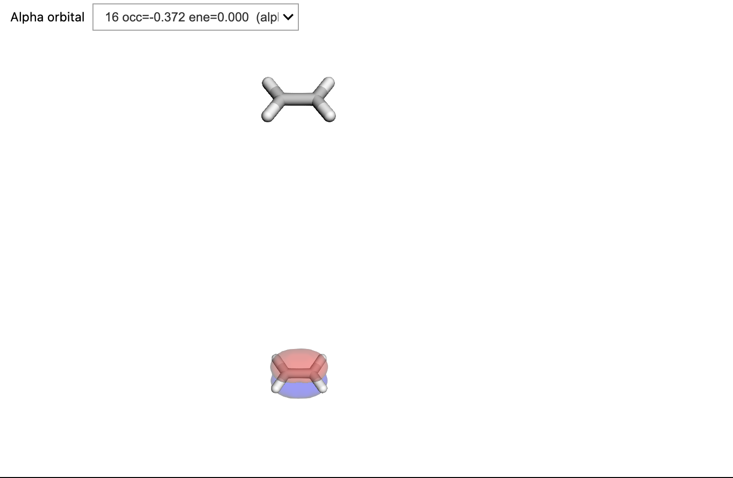

Implementation¶

Below follows an implementation of the NTO concept. First, we find the dimensions of the involved vectors and matrices.

norb = basis.get_dimension_of_basis()
nocc = molecule.number_of_alpha_electrons()
nvirt = norb - nocc
nexc = nocc * nvirt

print("Number of orbitals:", norb)
print("Number of occupied orbitals:", nocc)
print("Number of unoccupied orbitals:", nvirt)
print("Number of excitations:", nexc)

Number of orbitals: 52
Number of occupied orbitals: 16
Number of unoccupied orbitals: 36
Number of excitations: 576

The RPA eigenvector is obtained with use of the get_full_solution_vector() method and thereafter scattered into the transition matrix that becomes SVD factorized.

Xf = lreig_drv.get_full_solution_vector(
    lreig_results["eigenvectors_distributed"][state]
)

Zf = Xf[:nexc]
Yf = Xf[nexc:]
T = np.reshape(Zf - Yf, (nocc, nvirt))
U, L, V = np.linalg.svd(T)

print("Square of diagonal elements:\n", L**2)

Square of diagonal elements:
 [3.72487363e-01 3.72487363e-01 2.29200029e-02 2.29200028e-02
 6.24536155e-03 6.24536155e-03 4.88179212e-03 4.88179212e-03
 3.99368059e-03 3.99368059e-03 2.04378346e-03 2.04378346e-03
 4.29061774e-07 4.29061773e-07 3.18951957e-07 3.18951957e-07]

We note that these $\lambda$ -values are in perfect agreement with those obtained in the reference calculation.