Constrained coordinates

import veloxchem as vlx

We define a structure in terms of a SMILES string.

molecule = vlx.Molecule.read_smiles("OC=CC=O")
molecule.show(atom_indices=True)

We also define the electronic structure theory method to be used as well as an VeloxChem optimization driver.

scf_drv = vlx.XtbDriver()
scf_drv.ostream.mute()

opt_drv = vlx.OptimizationDriver(scf_drv)
opt_drv.ostream.mute()

Set and freeze internal coordinates¶

A selection of internal coordinates can be set or frozen during the molecular structure optimization, where the latter choice means that they are frozen to the values given in the initial structure. These options apply to internal coordinates of the types:

distance
angle
dihedral

opt_drv.constraints = [
    "set dihedral 6 1 2 3 0.0",
    "freeze distance 6 1",
]

opt_results = opt_drv.compute(molecule)

final_geometry = vlx.Molecule.read_xyz_string(opt_results["final_geometry"])
final_geometry.show()

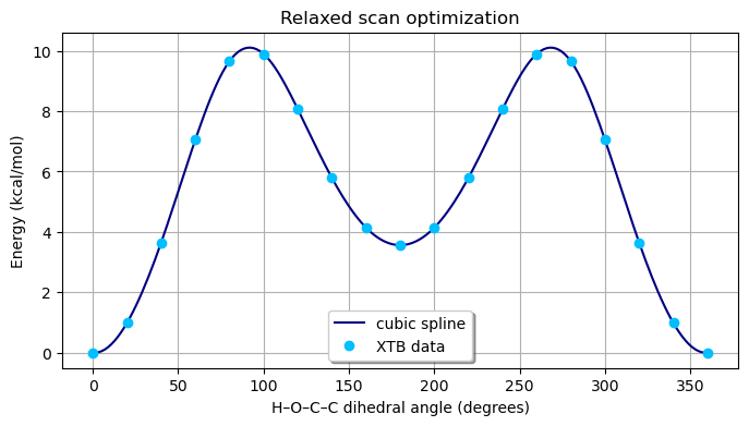
Scan internal coordinates¶

Relaxed scans of internal coordinates can be performed.

opt_drv.constraints = ["scan dihedral 6 1 2 3 0 360 19"]

opt_results = opt_drv.compute(molecule)

Energies and molecular structures are returned.

opt_results.keys()

dict_keys(['final_geometry', 'scan_energies', 'scan_geometries'])

Let us plot the potential energy curve from the relaxed scan structure optimization.

import numpy as np
import scipy

occc = np.linspace(0, 360, 19)

e_min_in_au = min(opt_results["scan_energies"])

energy_scan = [
    (e - e_min_in_au) * vlx.hartree_in_kcalpermol()
    for e in opt_results["scan_energies"]
]

spline_func = scipy.interpolate.interp1d(occc, energy_scan, kind="cubic")

x_spline = np.linspace(occc[0], occc[-1], 200)
y_spline = spline_func(x_spline)

from matplotlib import pyplot as plt

fig, ax = plt.subplots(figsize=(8, 4))

ax.plot(x_spline, y_spline, "-", color="navy", label="cubic spline")
ax.plot(occc, energy_scan, "o", color="deepskyblue", label="XTB data")

ax.legend(frameon=True, shadow=True, loc="lower center")

ax.grid(True)

ax.set_title("Relaxed scan optimization")
ax.set_xlabel("H–O–C–C dihedral angle (degrees)")
ax.set_ylabel("Energy (kcal/mol)")

plt.show()