Orbitals and densities

We here focus on the visualization of molecular orbitals and radial densities.

import matplotlib.pyplot as plt
import numpy as np
import py3Dmol
import veloxchem as vlx
import multipsi as mtp

Molecular orbitals¶

Using OrbitalViewer¶

Considering thymine with a minimal basis set, the SCF is optimized in order to provide the canonical orbitals.

thymine_xyz = """15
*
 C     0.095722    -0.037785    -1.093615
 C    -0.011848     1.408694    -1.113404
 C    -0.204706     2.048475     0.052807
 N    -0.302595     1.390520     1.249226
 C    -0.214596     0.023933     1.378238
 N    -0.017387    -0.607231     0.171757
 O     0.270287    -0.735594    -2.076393
 C     0.098029     2.096194    -2.424990
 H     1.052976     1.874860    -2.891573
 H     0.002157     3.170639    -2.310554
 H    -0.671531     1.743694    -3.104794
 O    -0.301905    -0.554734     2.440234
 H    -0.292790     3.119685     0.106201
 H     0.053626    -1.612452     0.215637
 H    -0.446827     1.892203     2.107092
"""

# Create veloxchem mol and basis objects
molecule = vlx.Molecule.read_xyz_string(thymine_xyz)
basis = vlx.MolecularBasis.read(molecule, "sto-3g", ostream=None)

# Perform SCF calculation
scf_drv = vlx.ScfRestrictedDriver()
scf_drv.ostream.mute()
scf_results = scf_drv.compute(molecule, basis)

molecule.show()

The resulting MOs can then be illustrated interactively with OrbitalViewer, which is available through the VeloxChem package:

viewer = vlx.OrbitalViewer()
viewer.plot(molecule, basis, scf_drv.mol_orbs)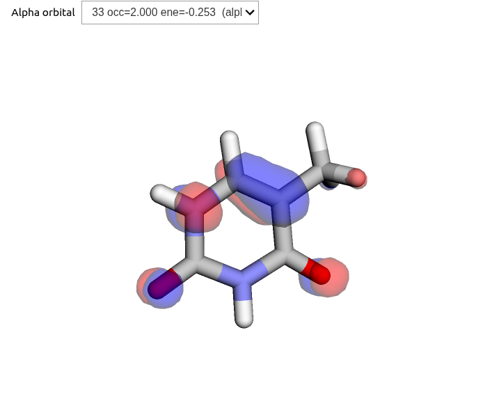

These routines are also available in the MultiPsi package, where additional functionalities for selecting and saving an active space are available:

viewer = mtp.OrbitalViewer()
viewer.plot(molecule, basis, scf_drv.mol_orbs)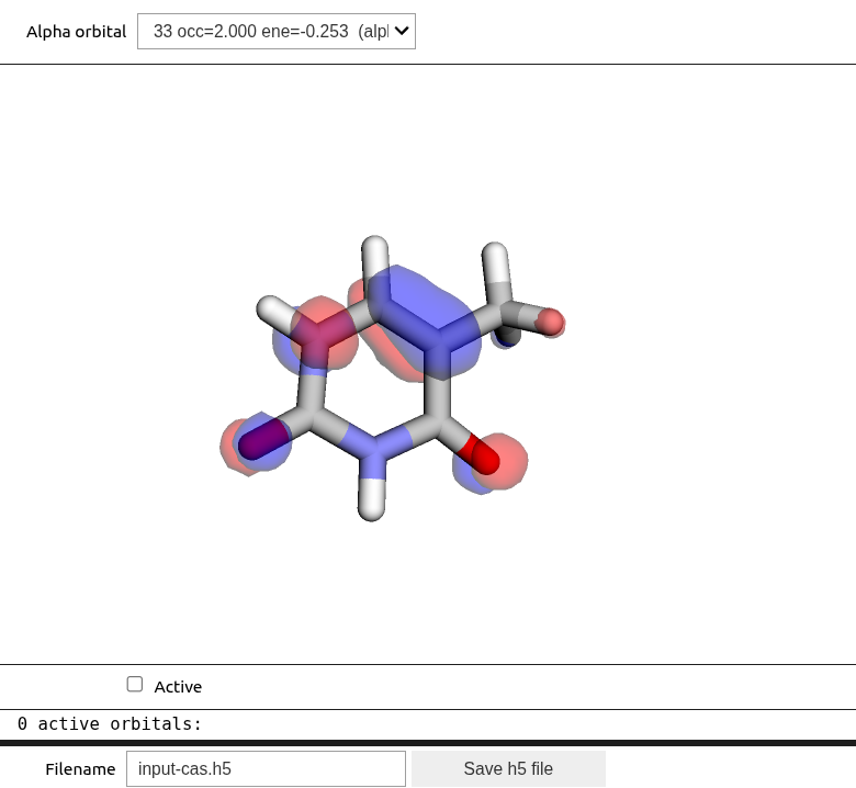

Using cube-files¶

Volumetric data can be constructed and saved using the VisualizationDriver, which can then be illustrated with py3Dmol. The file sizes can be quite substantial, and we thus recommend using more light-weight modules whenever possible.

The HOMO, LUMO, and $\alpha$ densities of water are constructed and saved as cube-files using:

water_mol_str = """
O       0.0000000000     0.0000000000     0.1178336003
H      -0.7595754146    -0.0000000000    -0.4713344012
H       0.7595754146     0.0000000000    -0.4713344012
"""

molecule = vlx.Molecule.read_molecule_string(water_mol_str)
basis = vlx.MolecularBasis.read(molecule, "6-31G", ostream=None)
vis_drv = vlx.VisualizationDriver()
scf_drv = vlx.ScfRestrictedDriver()
scf_drv.ostream.mute()

vis_drv.gen_cubes(
    cube_dict={
        "cubes": "mo(homo),mo(lumo),density(alpha)",
        "files": "../../img/visualize/water_HOMO.cube,../../img/visualize/water_LUMO.cube,../../img/visualize/water_a_density.cube",
    },
    molecule=molecule,
    basis=basis,
    mol_orbs=scf_drv.mol_orbs,
    density=scf_drv.density,
)

Overlaying the densities on stick structures, we obtain below results.

viewer = py3Dmol.view(linked=False, viewergrid=(1, 3), width=800, height=300)

# HOMO
with open("../../img/vis/water_HOMO.cube", "r") as f:
    cube = f.read()
# Plot strick structures
viewer.addModel(cube, "cube", viewer=(0, 0))
viewer.setStyle({"stick": {}}, viewer=(0, 0))
# Negative and positive nodes
viewer.addVolumetricData(
    cube, "cube", {"isoval": -0.02, "color": "blue", "opacity": 0.75}, viewer=(0, 0)
)
viewer.addVolumetricData(
    cube, "cube", {"isoval": 0.02, "color": "red", "opacity": 0.75}, viewer=(0, 0)
)
viewer.rotate(-45, "x", viewer=(0, 0))

# LUMO
with open("../../img/vis/water_LUMO.cube", "r") as f:
    cube = f.read()
viewer.addModel(cube, "cube", viewer=(0, 1))
viewer.setStyle({"stick": {}}, viewer=(0, 1))
viewer.addVolumetricData(
    cube, "cube", {"isoval": -0.02, "color": "blue", "opacity": 0.75}, viewer=(0, 1)
)
viewer.addVolumetricData(
    cube, "cube", {"isoval": 0.02, "color": "red", "opacity": 0.75}, viewer=(0, 1)
)
viewer.rotate(-45, "x", viewer=(0, 1))

# Alpha density
with open("../../img/vis/water_a_density.cube", "r") as f:
    cube = f.read()
viewer.addModel(cube, "cube", viewer=(0, 2))
viewer.setStyle({"stick": {}}, viewer=(0, 2))
viewer.addVolumetricData(
    cube, "cube", {"isoval": 0.02, "color": "red", "opacity": 0.75}, viewer=(0, 2)
)
viewer.rotate(-45, "x", viewer=(0, 2))

viewer.show()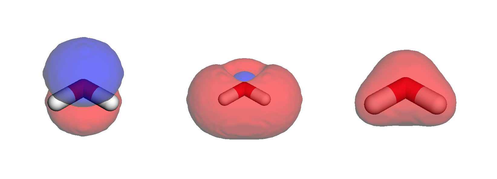

Radial distribution¶

In order to illustrate radial distributions, we consider the neon atom with a double-zeta basis set:

mol_str = """
Ne        0.00000000    0.00000000    0.00000000
"""
molecule = vlx.Molecule.read_molecule_string(mol_str)
basis = vlx.MolecularBasis.read(molecule, "cc-pVDZ", ostream=None)

scf_drv = vlx.ScfRestrictedDriver()
scf_drv.ostream.mute()
scf_results = scf_drv.compute(molecule, basis)

Valence orbitals¶

Considering the occupied MOs along the z-axis:

vis_drv = vlx.VisualizationDriver()

mol_orbs = scf_drv.mol_orbs
# define the coordinates (in Bohr) for which you wish values of orbitals
n = 100
coords = np.zeros((n, 3))
r = np.linspace(0, 2, n)
coords[:, 2] = r  # radial points along the z-axis

# get the values of orbitals
mo_alpha = mol_orbs.alpha_to_numpy()
mo_1s = np.array(vis_drv.get_mo(coords, molecule, basis, mo_alpha, 0))
mo_2s = np.array(vis_drv.get_mo(coords, molecule, basis, mo_alpha, 1))
mo_2p_1 = np.array(vis_drv.get_mo(coords, molecule, basis, mo_alpha, 2))
mo_2p_2 = np.array(vis_drv.get_mo(coords, molecule, basis, mo_alpha, 3))
mo_2p_3 = np.array(vis_drv.get_mo(coords, molecule, basis, mo_alpha, 4))

# adjust signs
mo_1s = np.sign(mo_1s[10]) * mo_1s
mo_2s = np.sign(mo_2s[10]) * mo_2s
mo_2p_1 = np.sign(mo_2p_1[10]) * mo_2p_1
mo_2p_2 = np.sign(mo_2p_2[10]) * mo_2p_2
mo_2p_3 = np.sign(mo_2p_3[10]) * mo_2p_3

fig = plt.figure(1, figsize=(8, 6))

plt.plot(r, mo_1s, r, mo_2s, r, mo_2p_1, r, mo_2p_2, r, mo_2p_3)

plt.axhline(y=0.0, color="0.5", linewidth=0.7, dashes=[3, 1, 3, 1])
plt.setp(plt.gca(), xlim=(0, 2), ylim=(-1, 6))
plt.legend(
    [r"$1s$", r"$2s$", r"$2p_1$", r"$2p_2$", r"$2p_3$"],
    loc="upper right",
    frameon=False,
)

plt.title(r"Valence orbitals of Neon")
plt.xlabel(r"Distance to nucleus (Bohr)")
plt.ylabel(r"Orbital value (a.u.)")

plt.show()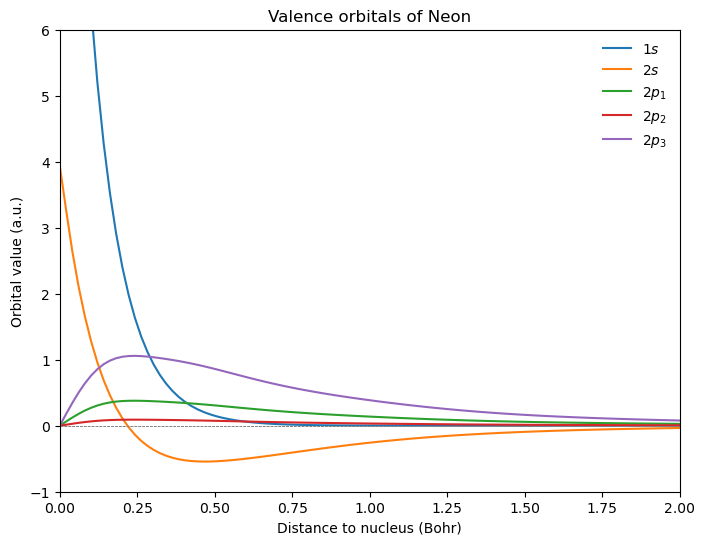

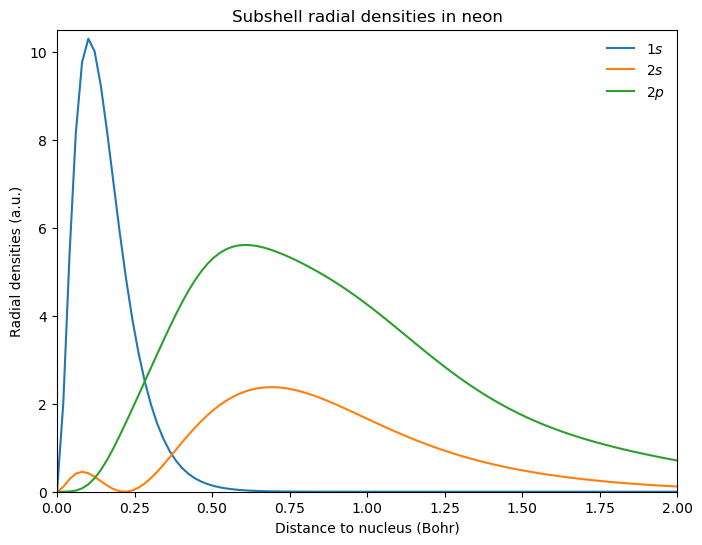
Atomic sub-shell densities¶

Looking at the densities of different sub-shells, we obtain:

fig = plt.figure(2, figsize=(8, 6))

# additional factor of 2 from alpha and beta spin orbitals
rad_den_1s = 4 * np.pi * r ** 2 * 2 * mo_1s ** 2
rad_den_2s = 4 * np.pi * r ** 2 * 2 * mo_2s ** 2
rad_den_2p = 4 * np.pi * r ** 2 * 2 * (mo_2p_1 ** 2 + mo_2p_2 ** 2 + mo_2p_3 ** 2)

plt.plot(r, rad_den_1s, r, rad_den_2s, r, rad_den_2p)

plt.axhline(y=0.0, color="0.5", linewidth=0.7, dashes=[3, 1, 3, 1])
plt.setp(plt.gca(), xlim=(0, 2), ylim=(0.0, 10.5))
plt.legend([r"$1s$", r"$2s$", r"$2p$"], loc="upper right", frameon=False)

plt.title(r"Subshell radial densities in neon")
plt.xlabel(r"Distance to nucleus (Bohr)")
plt.ylabel(r"Radial densities (a.u.)")

plt.show()