The following steps are carried out mostly by the geomeTRIC module Wang & Song (2016), hence they are described in less detail. For more details on the topic, the reader is referred to Molecular Vibrations by Wilson, Decius and Cross Wilson et al. (1980).
Cartesian and mass-weighted Hessian
The starting point for the vibrational analysis of molecules is the Hessian matrix in Cartesian coordinates, , calculated either numerically or analytically as described in the previous section. Generally, the elements of are given by second derivatives of the energy with respect to nuclear displacement
Hence, is a matrix (where is the number of atoms), and denote displacements of the Cartesian coordinates. The ‘0’ subscript indicates that the second derivatives are taken at the equilibrium geometry, where the first derivatives (or gradient) vanish.
As a first step, the Hessian is converted to mass-weighted Cartesian coordinates (MWC), , , , , where is the mass of atom , such that is given by
Diagonalizing this Hessian gives eigenvalues which represent the fundamental frequencies of the molecule, but include translation and rotational modes.
Translating and rotating frame
In order to remove translational and rotational degrees of freedom, one first determines the center of mass (COM) in the usual way
where the sum runs over all atoms , and the origin is then shifted to the COM, . Subsequently, one determines the inertia tensor and diagonalizes it to obtain principal moments and axes of inertia. Next, one needs to find the transformation from mass-weighted Cartesian coordinates to a set of coordinates, where the molecule’s translation and rotation are separated out, leaving (or for linear molecules) vibrational modes.
This is achieved by applying the so-called Eckart conditions Eckart (1935). While the three vectors of length corresponding to translation are simply given by times the coordinate axis, the vectors corresponding to rotational motion of the atoms are obtained from the coordinates of the atoms with respect to the COM and the corresponding row of the matrix used to diagonalize the moment of inertia tensor. In the next step, these vectors are normalized and a Gram--Schmidt orthogonalization is carried out to create (or ) remaining vectors, which are orthogonal to the five or six translational and rotational vectors. Thus, one obtains a transformation matrix which allows for the transformation of the mass-weighted Cartesian coordinates to internal coordinates , where translation and rotation have been projected out.
Hessian in internal coordinates and harmonic frequencies
Now the Hessian , which is still given in mass-weighted Cartesian coordinates, is transformed the the internal coordinate system,
yielding a representation in internal coordinates from the full Cartesian coordinates. The Hessian in internal coordinates is successively diagonalized,
where is the diagonal matrix of eigenvalues which are related to the harmonic vibrational frequencies and is the transformation matrix composed of the eigenvectors.
Finally, the eigenvalues can be converted from frequencies to wavenumbers in reciprocal centimeters by using the relationship , where is the speed of light.The wavenumbers are thus obtained from
and successively appropriate conversion factors are applied to obtain the wavenumbers in inverse centimeters (cm).
Cartesian displacements, reduced masses, and force constants
The Cartesian normal modes are obtained by combining this and this equation together with a diagonal matrix defined by to undo the mass-weighting, , with the individual elements of this matrix being given by
The (normalized) column vectors of correspond to the normal-mode displacements in Cartesian coordinates, which are used together with property gradients for the calculation of spectral intensities as described here.
From the Cartesian normal modes , the reduced mass of vibration can be calculated as
Using the reduced masses, the corresponding force constants are calculated as
since .
The spectral intensities are calculated from the dipole moment gradient (IR spectroscopy), or the polarizability gradient (Raman spectroscopy).
Practical example
We can perform a vibrational analysis using the VibrationalAnalysis class of VeloxChem. Let us create a molecule, optimize the geometry, and run the vibrational analysis on the optimized geometry.
import veloxchem as vlxmolecule = vlx.Molecule.read_smiles("C=C")
basis = vlx.MolecularBasis.read(molecule, "def2-svp")
scf_drv = vlx.ScfRestrictedDriver()
scf_drv.xcfun = "b3lyp"
scf_results = scf_drv.compute(molecule, basis)Output
                                            Self Consistent Field Driver Setup
                                           ====================================

                   Wave Function Model             : Spin-Restricted Kohn-Sham
                   Initial Guess Model             : Superposition of Atomic Densities
                   Convergence Accelerator         : Two Level Direct Inversion of Iterative Subspace
                   Max. Number of Iterations       : 50
                   Max. Number of Error Vectors    : 10
                   Convergence Threshold           : 1.0e-06
                   ERI Screening Threshold         : 1.0e-12
                   Linear Dependence Threshold     : 1.0e-06
                   Exchange-Correlation Functional : B3LYP
                   Molecular Grid Level            : 4

* Info * Using the B3LYP functional.

         P. J. Stephens, F. J. Devlin, C. F. Chabalowski, and M. J. Frisch.,  J. Phys. Chem. 98, 11623 (1994)

* Info * Using the Libxc library (v7.0.0).

         S. Lehtola, C. Steigemann, M. J.T. Oliveira, and M. A.L. Marques.,  SoftwareX 7, 1–5 (2018)

* Info * Using the following algorithm for XC numerical integration.

         J. Kussmann, H. Laqua and C. Ochsenfeld, J. Chem. Theory Comput. 2021, 17, 1512-1521

* Info * Starting Reduced Basis SCF calculation...
* Info * ...done. SCF energy in reduced basis set: -77.938548728100 a.u. Time: 0.05 sec.


               Iter. |    Kohn-Sham Energy | Energy Change | Gradient Norm | Max. Gradient | Density Change
               --------------------------------------------------------------------------------------------
                  1       -78.527729546789    0.0000000000      0.14829775      0.01829952      0.00000000
                  2       -78.528666291263   -0.0009367445      0.12722270      0.01641138      0.09743158
                  3       -78.530925966573   -0.0022596753      0.00111586      0.00018436      0.04032517
                  4       -78.530926171342   -0.0000002048      0.00015835      0.00002056      0.00060949
                  5       -78.530926174550   -0.0000000032      0.00002815      0.00000316      0.00006271
                  6       -78.530926174666   -0.0000000001      0.00000229      0.00000034      0.00001445
                  7       -78.530926174666   -0.0000000000      0.00000086      0.00000012      0.00000097

               *** SCF converged in 7 iterations. Time: 0.86 sec.

               Spin-Restricted Kohn-Sham:
               --------------------------
               Total Energy                       :      -78.5309261747 a.u.
               Electronic Energy                  :     -111.9453361984 a.u.
               Nuclear Repulsion Energy           :       33.4144100238 a.u.
               ------------------------------------
               Gradient Norm                      :        0.0000008637 a.u.


               Ground State Information
               ------------------------
               Charge of Molecule            :  0.0
               Multiplicity (2S+1)           :  1
               Magnetic Quantum Number (M_S) :  0.0
opt_drv = vlx.OptimizationDriver(scf_drv)
opt_results = opt_drv.compute(molecule, basis, scf_results)
Output
opt_molecule = vlx.Molecule.read_xyz_string(opt_results['final_geometry'])
opt_molecule.show()vib_analysis = vlx.VibrationalAnalysis(scf_drv)
vib_analysis_results = vib_analysis.compute(opt_molecule, basis)Output
Vibrational Analysis Driver
=============================
The following will be computed:
- Vibrational frequencies and normal modes
- Force constants
- IR intensities
SCF Hessian Driver Setup
==========================
Hessian Type : Analytical
* Info * Computing analytical Hessian...
Reference: P. Deglmann, F. Furche, R. Ahlrichs, Chem. Phys. Lett. 2002, 362, 511-518.
* Info * Using the B3LYP functional.
P. J. Stephens, F. J. Devlin, C. F. Chabalowski, and M. J. Frisch., J. Phys. Chem. 98, 11623 (1994)
* Info * Using the Libxc library (v7.0.0).
S. Lehtola, C. Steigemann, M. J.T. Oliveira, and M. A.L. Marques., SoftwareX 7, 1–5 (2018)
* Info * Using the following algorithm for XC numerical integration.
J. Kussmann, H. Laqua and C. Ochsenfeld, J. Chem. Theory Comput. 2021, 17, 1512-1521
* Info * CPHF/CPKS integral derivatives computed in 1.41 sec.
* Info * CPHF/CPKS right-hand side computed in 1.67 sec.
Coupled-Perturbed Kohn-Sham Solver Setup
------------------------------------------
Solver Type : Iterative Subspace Algorithm
Max. Number of Iterations : 150
Convergence Threshold : 1.0e-04
Exchange-Correlation Functional : B3LYP
Molecular Grid Level : 4
* Info * 15 trial vectors in reduced space
*** Iteration: 1 * Residuals (Max,Min): 3.45e-01 and 8.99e-02
* Info * 30 trial vectors in reduced space
*** Iteration: 2 * Residuals (Max,Min): 2.94e-02 and 9.09e-03
* Info * 45 trial vectors in reduced space
*** Iteration: 3 * Residuals (Max,Min): 2.28e-03 and 5.60e-04
* Info * 57 trial vectors in reduced space
*** Iteration: 4 * Residuals (Max,Min): 2.01e-04 and 2.67e-05
* Info * 66 trial vectors in reduced space
*** Iteration: 5 * Residuals (Max,Min): 2.67e-05 and 9.37e-06
* Info * Checkpoint written to file: vlx_20260408_e29164fb_orbrsp.h5
* Info * Time spent in writing checkpoint file: 0.01 sec
*** Coupled-Perturbed Kohn-Sham converged in 5 iterations. Time: 8.35 sec
* Info * First order derivative contributions to the Hessian computed in 0.00 sec.
* Info * Second order derivative contributions to the Hessian computed in 10.54 sec.
*** Time spent in Hessian calculation: 18.93 sec ***
Free Energy Analysis
======================
Note: Rotational symmetry is set to 1 regardless of true symmetry
No Imaginary Frequencies
Free energy contributions calculated at @ 298.15 K:
Zero-point vibrational energy: 31.8098 kcal/mol
H (Trans + Rot + Vib = Tot): 1.4812 + 0.8887 + 0.1364 = 2.5063 kcal/mol
S (Trans + Rot + Vib = Tot): 35.9530 + 18.6437 + 0.5555 = 55.1523 cal/mol/K
TS (Trans + Rot + Vib = Tot): 10.7194 + 5.5586 + 0.1656 = 16.4437 kcal/mol
Ground State Electronic Energy : E0 = -78.53159665 au ( -49279.3209 kcal/mol)
Free Energy Correction (Harmonic) : ZPVE + [H-TS]_T,R,V = 0.02848167 au ( 17.8725 kcal/mol)
Gibbs Free Energy (Harmonic) : E0 + ZPVE + [H-TS]_T,R,V = -78.50311498 au ( -49261.4484 kcal/mol)
Vibrational Analysis
======================
* Info * The 5 dominant normal modes are printed below.
Vibrational Mode 1
----------------------------------------------------
Harmonic frequency: 822.33 cm**-1
Reduced mass: 1.0423 amu
Force constant: 0.4153 mdyne/A
IR intensity: 0.7353 km/mol
Normal mode:
X Y Z
1 C -0.0138 0.0177 -0.0327
2 C -0.0138 0.0177 -0.0327
3 H -0.2292 -0.4143 0.1585
4 H 0.3932 0.2036 0.2305
5 H -0.2292 -0.4143 0.1585
6 H 0.3932 0.2036 0.2305
Vibrational Mode 2
----------------------------------------------------
Harmonic frequency: 965.12 cm**-1
Reduced mass: 1.1607 amu
Force constant: 0.6370 mdyne/A
IR intensity: 82.5824 km/mol
Normal mode:
X Y Z
1 C 0.0513 -0.0463 -0.0467
2 C 0.0513 -0.0463 -0.0467
3 H -0.3057 0.2755 0.2781
4 H -0.3055 0.2753 0.2779
5 H -0.3057 0.2755 0.2781
6 H -0.3054 0.2753 0.2779
Vibrational Mode 7
----------------------------------------------------
Harmonic frequency: 1443.73 cm**-1
Reduced mass: 1.1119 amu
Force constant: 1.3655 mdyne/A
IR intensity: 6.6103 km/mol
Normal mode:
X Y Z
1 C -0.0487 -0.0483 -0.0056
2 C -0.0487 -0.0483 -0.0056
3 H 0.1916 0.4137 -0.1993
4 H 0.3880 0.1616 0.2664
5 H 0.1916 0.4137 -0.1993
6 H 0.3880 0.1616 0.2664
Vibrational Mode 9
----------------------------------------------------
Harmonic frequency: 3124.29 cm**-1
Reduced mass: 1.0477 amu
Force constant: 6.0257 mdyne/A
IR intensity: 13.3681 km/mol
Normal mode:
X Y Z
1 C 0.0301 0.0299 0.0034
2 C 0.0301 0.0299 0.0034
3 H -0.3286 0.0137 -0.3749
4 H -0.0300 -0.3703 0.3338
5 H -0.3287 0.0137 -0.3749
6 H -0.0300 -0.3703 0.3338
Vibrational Mode 12
----------------------------------------------------
Harmonic frequency: 3234.02 cm**-1
Reduced mass: 1.1181 amu
Force constant: 6.8899 mdyne/A
IR intensity: 18.3295 km/mol
Normal mode:
X Y Z
1 C 0.0246 -0.0316 0.0584
2 C 0.0246 -0.0316 0.0584
3 H -0.3336 0.0029 -0.3695
4 H 0.0401 0.3733 -0.3258
5 H -0.3336 0.0029 -0.3695
6 H 0.0401 0.3733 -0.3258
Once the vibrational analysis has been performed, we can animate the vibrational normal modes, or plot the IR spectrum.
vib_analysis.animate(vib_analysis_results, mode=1)vib_analysis.plot(vib_results=vib_analysis_results)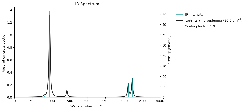
- Wang, L.-P., & Song, C. (2016). Geometry optimization made simple with translation and rotation coordinates. J. Chem. Phys., 144, 214108. 10.1063/1.4952956
- Wilson, E. B., Decius, J. C., & Cross, P. C. (1980). Molecular Vibrations. Dover, New York.
- Eckart, C. (1935). Some Studies Concerning Rotating Axes and Polyatomic Molecules. Phys. Rev., 47, 552–558. 10.1103/PhysRev.47.552