Here we provide quick reference calculation for some of the most common X-ray spectrum calculations, considering XPS/IE, XAS, and (non-resonant) XES of water, as well as a typical workflow.
Typical workflow
Perform structure optimization
Calculate the spectra/ionization energies
Choose suitable level of theory
Depending on spectroscopy:
Ionization energy: using -methods, or target transitions to extremely diffuse MOs
XES: ADC, TDSCF, and using ground state MOs
Analysis and assignment of the spectra
Looking at amplitudes
Visualization
IEs and XPS
Koopmans’ theorem
While it is not recommended for any production calculations, estimates of ionization energies can be obtained from Koopmans’ theorem:
import numpy as np
import veloxchem as vlx

# for vlx
silent_ostream = vlx.OutputStream(None)
from mpi4py import MPI

comm = MPI.COMM_WORLD
# au to eV conversion factor
au2ev = 27.211386

water_mol_str = """
O       0.0000000000     0.0000000000     0.1178336003
H      -0.7595754146    -0.0000000000    -0.4713344012
H       0.7595754146     0.0000000000    -0.4713344012
"""

# Create veloxchem mol and basis objects
mol_vlx = vlx.Molecule.read_molecule_string(water_mol_str)
bas_vlx = vlx.MolecularBasis.read(mol_vlx, "6-31G")

# Perform SCF calculation
scf_gs = vlx.ScfRestrictedDriver(comm, ostream=silent_ostream)
scf_results = scf_gs.compute(mol_vlx, bas_vlx)

# Extract orbital energies
orbital_energies = scf_results["E_alpha"]
print("1s E from Koopmans' theorem:", np.around(au2ev * orbital_energies[0], 2), "eV")1s E from Koopmans' theorem: -559.5 eV
-methods
Substantially improved ionization energies are obtained using -methods, where the energy difference of the ground state and core-hole state is used to estimate the IE:
import copy

import numpy as np
from pyscf import gto, mp, scf

water_xyz = """
O       0.0000000000     0.0000000000     0.1178336003
H      -0.7595754146    -0.0000000000    -0.4713344012
H       0.7595754146     0.0000000000    -0.4713344012
"""

# Create pyscf mol object
mol = gto.Mole()
mol.atom = water_xyz
mol.basis = "6-31G"
mol.build()

# Perform unrestricted SCF calculation
scf_gs = scf.UHF(mol)
scf_gs.kernel()

# Copy molecular orbitals and occupations
mo0 = copy.deepcopy(scf_gs.mo_coeff)
occ0 = copy.deepcopy(scf_gs.mo_occ)

# Create 1s core-hole by setting alpha_0 population to zero
occ0[0][0] = 0.0

# Perform unrestricted SCF calculation with MOM constraint
scf_ion = scf.UHF(mol)
scf.addons.mom_occ(scf_ion, mo0, occ0)
scf_ion.kernel()

# Run MP2 on neutral and core-hole state
mp_res = mp.MP2(scf_gs).run()
mp_ion = mp.MP2(scf_ion).run()

# IE from energy difference
print(
    "HF ionization energy:",
    np.around(au2ev * (scf_ion.energy_tot() - scf_gs.energy_tot()), 2),
    "eV",
)
print(
    "MP2 ionzation energy:", np.around(au2ev * (mp_ion.e_tot - mp_res.e_tot), 2), "eV"
)import gator
import matplotlib.pyplot as plt
water_mol_str = """
O 0.0000000000 0.0000000000 0.1178336003
H -0.7595754146 -0.0000000000 -0.4713344012
H 0.7595754146 0.0000000000 -0.4713344012
"""
# Construct structure and basis objects
struct = gator.get_molecule(water_mol_str)
basis = gator.get_molecular_basis(struct, "6-31G")
# Perform SCF calculation
scf_gs = gator.run_scf(struct, basis)
# Calculate the 6 lowest eigenstates with CVS restriction to MO #1 (oxygen 1s)
adc_res = gator.run_adc(
struct, basis, scf_gs, method="cvs-adc2x", singlets=4, core_orbitals=1
)# Print information on eigenstates
print(adc_res.describe())
plt.figure(figsize=(6, 5))
# Convolute using functionalities available in gator and adcc
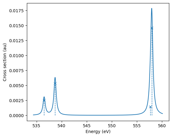
adc_res.plot_spectrum()
plt.show()+--------------------------------------------------------------+
| cvs-adc2x singlet , converged |
+--------------------------------------------------------------+
| # excitation energy osc str |v1|^2 |v2|^2 |
| (au) (eV) |
| 0 19.71638 536.5099 0.0178 0.8 0.2 |
| 1 19.7967 538.6956 0.0373 0.8087 0.1913 |
| 2 20.49351 557.6567 0.0099 0.7858 0.2142 |
| 3 20.50482 557.9647 0.1016 0.8441 0.1559 |
+--------------------------------------------------------------+
CPP-DFT
To be added
XES
ADC
The non-resonant X-ray emission spectrum can be calculated with a two-step approach using ADC:
import copy

import adcc
import matplotlib.pyplot as plt
import numpy as np
from pyscf import gto, mp, scf

water_xyz = """
O       0.0000000000     0.0000000000     0.1178336003
H      -0.7595754146    -0.0000000000    -0.4713344012
H       0.7595754146     0.0000000000    -0.4713344012
"""

# Create pyscf mol object
mol = gto.Mole()
mol.atom = water_xyz
mol.basis = "6-31G"
mol.build()

# Perform unrestricted SCF calculation
scf_res = scf.UHF(mol)
scf_res.kernel()

# Copy molecular orbitals
mo0 = copy.deepcopy(scf_res.mo_coeff)
occ0 = copy.deepcopy(scf_res.mo_occ)

# Create 1s core-hole by setting alpha_0 population to zero
occ0[0][0] = 0.0

# Perform unrestricted SCF calculation with MOM constraint
scf_ion = scf.UHF(mol)
scf.addons.mom_occ(scf_ion, mo0, occ0)
scf_ion.kernel()

# Perform ADC calculation
adc_xes = adcc.adc2(scf_ion, n_states=4)

# Print information on eigenstates
print(adc_xes.describe())

plt.figure(figsize=(6, 5))
# Convolute using functionalities available in gator and adcc
adc_xes.plot_spectrum()
plt.show()