K-means clustering - Mathematical Modeling in Biotechnology

The clustering objective¶

K-means partitions a data set into $K$ clusters, each represented by a centroid $\boldsymbol{\mu}_k$ (the mean of all points assigned to that cluster), by minimizing the total within-cluster variance,

J = \sum_{k=1}^{K} \sum_{\boldsymbol{x}_i \in C_k} \lVert \boldsymbol{x}_i - \boldsymbol{\mu}_k \rVert^2

(1)

where $C_k$ is the set of points assigned to cluster $k$ . Unlike the supervised methods covered so far, K-means is unsupervised: there are no target labels $y$ to predict — the goal is to discover structure in the data itself.

The algorithm¶

Equation (1) is minimized by iterating two steps (Lloyd’s algorithm):

Assignment step. Assign every point to its nearest centroid: $c_i = \arg\min_k \lVert \boldsymbol{x}_i - \boldsymbol{\mu}_k \rVert^2$ .
Update step. Recompute each centroid as the mean of its assigned points: $\boldsymbol{\mu}_k = \frac{1}{|C_k|}\sum_{\boldsymbol{x}_i \in C_k} \boldsymbol{x}_i$ .

Each step can only decrease the objective $J$ , so convergence is guaranteed — but only to a local minimum that depends on the initial centroid positions.

Library imports¶

import matplotlib.pyplot as plt
import sklearn

Data preparation¶

We use the wine data set: 178 wine samples from three Italian cultivars, described by 13 chemical measurements. The task is to ask whether an unsupervised algorithm, given only the chemistry and no cultivar labels, can recover the three groups on its own.

The features must be standardized before applying K-means because Eq. (1) is Euclidean-distance based, so features with large numerical range would otherwise dominate the cluster assignments.

wine = sklearn.datasets.load_wine()
X, y_true = wine.data, wine.target

scaler = sklearn.preprocessing.StandardScaler()
X_scaled = scaler.fit_transform(X)

print("Number of samples :", X.shape[0])
print("True class counts :", {n: (y_true == i).sum() for i, n in enumerate(wine.target_names)})

Number of samples : 178
True class counts : {np.str_('class_0'): np.int64(59), np.str_('class_1'): np.int64(71), np.str_('class_2'): np.int64(48)}

Choosing the number of clusters: the elbow method¶

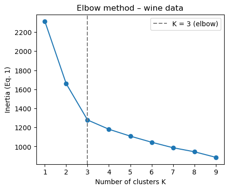
In real applications the true number of clusters is generally unknown. A common heuristic is the elbow method: fit K-means for a range of $K$ values and plot the resulting inertia (Eq. (1)), looking for the point where adding more clusters stops giving a large improvement.

inertias = []
K_range = range(1, 10)

for K in K_range:
    km = sklearn.cluster.KMeans(n_clusters=K, n_init=20, random_state=0)
    km.fit(X_scaled)
    inertias.append(km.inertia_)

plt.figure(figsize=(5, 4))
plt.plot(K_range, inertias, "o-")
plt.axvline(3, color="gray", linestyle="--", label="K = 3 (elbow)")
plt.xlabel("Number of clusters K")
plt.ylabel("Inertia (Eq. 1)")
plt.legend(); plt.title("Elbow method – wine data")
plt.show()

Model definition and training¶

The elbow at $K=3$ matches the three cultivars in the data. We fit the final model and retrieve the cluster labels.

kmeans = sklearn.cluster.KMeans(n_clusters=3, n_init=20, random_state=0)
kmeans.fit(X_scaled)
labels = kmeans.labels_

Evaluation¶

Since clustering provides no labels to compare against in a real application, we use two internal/external metrics. The silhouette score measures how similar each point is to its own cluster versus neighbouring clusters (range $[-1, 1]$ , higher is better) and needs no ground truth. The adjusted Rand index (ARI) measures agreement with the true cultivar labels and is included here because we happen to have them; in a real unsupervised setting only the silhouette score would be available.

sil = sklearn.metrics.silhouette_score(X_scaled, labels)
ari = sklearn.metrics.adjusted_rand_score(y_true, labels)
print(f"Silhouette score : {sil:.3f}")
print(f"Adjusted Rand index (vs. cultivar labels): {ari:.3f}")

Silhouette score : 0.285
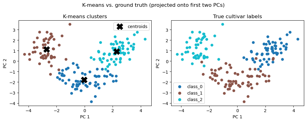
Adjusted Rand index (vs. cultivar labels): 0.897

Visualize in PCA space¶

We project the data onto the first two principal components to visualize the cluster assignments in 2D.

pca = sklearn.decomposition.PCA(n_components=2)
X_2d = pca.fit_transform(X_scaled)

fig, axes = plt.subplots(1, 2, figsize=(10, 4))
# K-means assignments
axes[0].scatter(X_2d[:, 0], X_2d[:, 1], c=labels, cmap="tab10", s=30)
centroids_2d = pca.transform(kmeans.cluster_centers_)
axes[0].scatter(centroids_2d[:, 0], centroids_2d[:, 1],
                marker="X", s=200, color="black", label="centroids")
axes[0].set_title("K-means clusters"); axes[0].legend()
# True cultivar labels
sc = axes[1].scatter(X_2d[:, 0], X_2d[:, 1], c=y_true, cmap="tab10", s=30)
for label, name in enumerate(wine.target_names):
    axes[1].scatter([], [], color=sc.cmap(sc.norm(label)), label=name)
axes[1].set_title("True cultivar labels"); axes[1].legend()
for ax in axes:
    ax.set_xlabel("PC 1"); ax.set_ylabel("PC 2")
plt.suptitle("K-means vs. ground truth (projected onto first two PCs)")
plt.tight_layout()
plt.show()

Cross-validation and model selection¶

$K$ is the main hyperparameter to tune. In the absence of ground-truth labels the silhouette score is the standard criterion: fit K-means for several values of $K$ and choose the one that maximizes it. For larger data sets sklearn.model_selection.KFold can also be used to get a stable estimate of the silhouette score across subsets of the data.

Take-away¶

K-means is fast, simple, and a good default choice for exploratory clustering with limited resources. Its main limitations are that it requires choosing $K$ in advance, assumes roughly spherical and similarly-sized clusters (because Eq. (1) uses the Euclidean distance to a single centroid per cluster), and can converge to different local minima depending on initialization — sklearn mitigates the last issue by running the algorithm several times (n_init) and keeping the best result.