Neural networks - Mathematical Modeling in Biotechnology

Components and structure¶

Neural networks are built as layers of neurons (also referred to as perceptrons). Every neuron has an associated activation level (a real number) representing its state. The activation level of neuron $n$ in layer $L$ is denoted $a^{(L)}_n$ .

The first and last layers are referred to as the input and output layers, respectively, and those in between are called hidden layers.

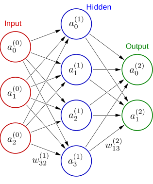
The input layer receives input data; hidden layers transform the data; and the output layer provides the results upon which model predictions are made.

Forward propagation¶

The input level apart, activation levels in a given level, say $L$ , are determined from those in the previous layer by use of weights that are collected in a matrix $\boldsymbol{W}^{(L)}$ and biases that are collected in a vector $\boldsymbol{b}^{(L)}$ .

The organization of the weights into matrix form is illustrated in the figure above. The neuron number in layer $L$ becomes the row index and the neuron number in layer $L-1$ becomes the column index.

A layer is referred to as linear if the weights and biases are applied in a linear transformation

\boldsymbol{a}^{(L)} = f(\boldsymbol{W}^{(L)} \boldsymbol{a}^{(L-1)} + \boldsymbol{b}^{(L)})

(1)

As indicated, to get the final activation levels also involves the elementwise operation of a (typically) nonlinear activation function, $f$ .

Activation functions¶

Several activation functions are available in the sklearn library.

For the hidden layers, users can choose from the following functions.

Activation	Formula	Range	Typical use
identity	x	(-∞, ∞)	rarely used
logistic	sigmoid	(0, 1)	older models
tanh	tanh	(-1, 1)	better than sigmoid
relu	max(0, x)	[0, ∞)	default/recommended

The output layer uses a predefined activation suited to the classification task.

Location	Activation options
Hidden layers	identity, logistic, tanh, relu
Output layer	logistic (binary), softmax (multiclass)

Sklearn libary import¶

We will make use of the sklearn library to build, train, and run multilayer perceptron (MLP) models.

import sklearn

Data preparation¶

Import data¶

Let us load the breast cancer data set, containing 569 data samples with 30 features. The target data is equal to 0 (malignant) or 1 (benign).

cancer = sklearn.datasets.load_breast_cancer()

X, y = cancer["data"], cancer["target"]

# Count number of benign and malignant tumors
number_benign = df[df["target"] == 1.0].shape[0]
number_malign = df[df["target"] == 0.0].shape[0]

print("Number benign   :", number_benign)
print("Number malignant:", number_malign)
print(21 * "-")
print("Total number    :", df.shape[0])

Number benign   : 357
Number malignant: 212
---------------------
Total number    : 569

Split data into training, validation, and test sets¶

Data are split into different categories.

Dataset	Purpose
Training data	Learn model parameters
Validation data	Tune model (hyperparameters, topology, etc.)
Test data	Final, unbiased evaluation

We will omit the category of validation data, and split the data into 80% training and 20% test data.

X_train, X_test, y_train, y_test = sklearn.model_selection.train_test_split(
    X,
    y,
    test_size=0.20,
    stratify=y,
)

With stratify activated, the training and test sets will get the same proportion of data classes (in this case malignant/benign).

Scale transformation of data¶

We scale all input features of the training data so they have mean 0 and standard deviation 1, which is essential for stable and efficient training of neural networks. The scaling parameters $\mu$ and $\sigma$ are computed for the training data and applied to both sets as to avoid using any information of the test set.

The transformation reads

X_\mathrm{scaled} = \frac{X - \mu}{\sigma}

(2)

scaler = sklearn.preprocessing.StandardScaler()

X_train_scaled = scaler.fit_transform(X_train)
X_test_scaled = scaler.transform(X_test)

This scaling results in the model putting equal focus on all features in the data set.

After the transformation, the training data becomes equal to

Network topology (or architecture)¶

We initialize an instance of the MLP classifier with 3 hidden layers (each with 8 nodes) and ReLU activation.

mlp = sklearn.neural_network.MLPClassifier(
    hidden_layer_sizes=(8, 8, 8),
    activation="relu",
    solver="adam",
    max_iter=500,
)

In our case, we have 30 features in the input layer and a single binary neuron in the output layer. The number of parameters in the model becomes:

(30 \times 8 + 8) + 2 \times (8 \times 8 + 8) + (8 + 1) = 401

(3)

Network architecture design is a bit of an art form. Some guiding principles include:

Begin with a small network and only increase size if needed.
The topology cannot be theoretically chosen:
- Shallow + wide networks are good for simpler tasks
- Deeper networks are better for:
  - data with complex hierarchical structures
  - high-dimensional data
Model size should scale with dataset size

Model	Training error	Validation error
Too small	high	high
Good	low	low
Too large	very low	high

Model training¶

By model training, we refer to the iterative process of changing the weight and bias parameters such that the output for the training data best reproduces the ground truth, i.e., the known results in supervised learning.

An epoch is one full pass through the training data. In MLP model optimization, an iteration corresponds to an epoch.

Loss function and parameter optimization¶

A loss function quantifies the discrepancy between model predictions and the true targets, guiding the learning process by providing a signal after which to adjust the model parameters.

MLPClassifier uses cross-entropy loss (log-loss), paired with sigmoid or softmax depending on the classification task.

mlp.fit(X_train_scaled, y_train)

After model training is performed, the number of parameters is available from model attributes.

for i, (W, b) in enumerate(zip(mlp.coefs_, mlp.intercepts_)):
    print(f"Layer {i}: weights = {W.shape}, biases = {b.shape}")

n_params = sum(w.size for w in mlp.coefs_) + sum(b.size for b in mlp.intercepts_)
print("Number of parameters:", n_params)

Layer 0: weights = (30, 8), biases = (8,)
Layer 1: weights = (8, 8), biases = (8,)
Layer 2: weights = (8, 8), biases = (8,)
Layer 3: weights = (8, 1), biases = (1,)
Number of parameters: 401

Model evaluation¶

The test data are used for model evaluation. The model should not have seen the test data prior to the evaluation.

y_pred = mlp.predict(X_test_scaled)

Classification report¶

print(sklearn.metrics.classification_report(y_test, y_pred, target_names=cancer["target_names"]))

              precision    recall  f1-score   support

   malignant       0.98      1.00      0.99        42
      benign       1.00      0.99      0.99        72

    accuracy                           0.99       114
   macro avg       0.99      0.99      0.99       114
weighted avg       0.99      0.99      0.99       114

Precision refers to the number of correct predictions (columns in the confusion matrix). Recall refers to the number of captured class targets (rows in the confusion matrix). The f1-score is the harmonic mean of precision and recall.

Confusion matrix¶

import matplotlib.pyplot as plt

cm = sklearn.metrics.confusion_matrix(y_test, y_pred)

disp = sklearn.metrics.ConfusionMatrixDisplay(confusion_matrix=cm, display_labels=cancer["target_names"])
disp.plot(cmap=plt.cm.Blues)

plt.title("MLP Confusion Matrix")
plt.show()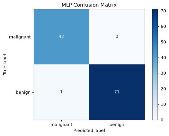

Additional material¶

A series of four videos on neural networks from the (generally) excellent channel 3Blue1Brown.