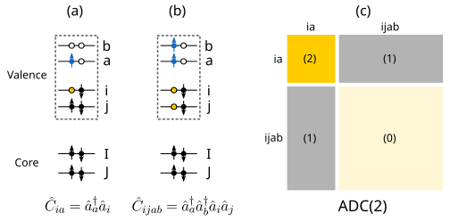
As the name suggest, the intermediate state representation (ISR) approach consists of constructing the ADC matrix with the help of intermediate states ∣Ψ~I⟩, obtained by applying excitation operators to the ground state ∣0⟩. In second quantization, the excitation operator is written as
where the indices a,b... refer to unoccupied orbitals, while i,j... represent occupied orbitals Schirmer (1991)Mertins & Schirmer (1996)Schirmer & Trofimov (2004). Schematic representations of single and double excitations, which are the only two excitation classes that are needed for ADC up to third order in perturbation theory, are depicted, with (a) single excitations, (b) double excitations, and (c) the structure of the ADC(2) matrix. The numbers in parenthesis indicate the highest order of perturbation theory used to describe each particular block.
The intermediate states ∣Ψ~I⟩ are obtained by first applying C^I to the many-body ground state
and then performing a Gram--Schmidt orthogonalization procedure with respect to lower excitation classes (including the ground state) to obtain precursor states ∣ΨI#⟩, which can then be orthonormalized symmetrically according to Wenzel (2016)
the solution of which yields vertical excitation energies (ωn=En−E0) as eigenvalues, collected in the diagonal matrix Ω, and the corresponding excitation vectors as eigenvectors Yn, collected in the columns of Y.
Having obtained an expression for the ADC matrix, we return to the series expansion of the polarization propagator. In the same way as the propagator is expanded in series, also the matrix elements can be written in terms of orders of perturbation Wenzel (2016)
where k and m are the orders of perturbation theory used for the overlap matrices SIK and SLJ, l is the order used for the matrix elements of the shifted Hamiltonian in the basis of precursor states, and the sum k+l+m=n represents the order of the contribution to the ADC matrix M. In order to get all contributions of a given order n, one needs to sum k,l,m over all terms for which k+l+m=n.
The effective transition amplitudes f can analogously be obtained in the ISR via
and the transition density matrices or transition amplitudes x by contracting with the eigenvectors,
x=Y†f.
Note that since f is a transition amplitude and not an expectation value,
it is not symmetric: fI,pq=fI,qp.
where the subscript denote the corresponding subblocks of the ADC matrix and XS is the singles part of the eigenvector.
From this, the order structure of the ADC matrix can be explained as follows.
The leading contributions of MSS and MDD, and thus also of (ω1−MDD)−1, are of zeroth order, whereas the leading contributions of MSD
and MDS are of first order.
Hence, if excited states dominated by single excitations are desired through, say, second order, then Meff
needs to be correct through this order, meaning that MSS needs to be correct through second order,
MSD and MDS need to be correct through first order,
whereas MDD only needs to be correct through zeroth order.
Expanding MDD through first order would lead to a third-order term
since the coupling blocks are at least of first order.
Equivalently, expanding the coupling blocks through second order would lead to third-order terms,
which are neglected in a second-order scheme.
A consistent third-order method requires each block one
order higher in perturbation theory, i.e. the singles-singles block through third oder, the
coupling blocks through second order and the doubles-doubles block through first order.
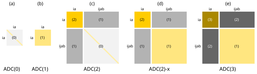
These findings are depicted schematically below
for ADC(n) schemes up to third order.
ADC(2)-x represents an ad hoc extension of ADC(2), where the first-order terms in the doubles-doubles block
from ADC(3) are taken into account in order to improve the description of doubly excited states.
However, this generally leads to an imbalanced description of singly and doubly excited states Dreuw & Wormit (2015).
The structure of the ADC(n) matrix at different orders n is illustrated below. The numbers indicate the orders of perturbation theory used to expand
the corresponding block.
Using above expansion of MIJ in combination with specific classes of excitation operators and truncating the series at the desired order, various levels of ADC theory are obtained. One aspect to note is that the excitation classes needed to construct a specific ADC level are directly connected to the order of perturbation theory. This can be easily seen in this illustration of the polarization propagator, where the zeroth and first order terms are related to single excitations (only one particle-hole pair is involved), while second order terms involve double excitations (two particle-hole pairs are involved). To illustrate this further, we list the explicit expressions for the ADC matrix M in spin-orbitals up to second order Wenzel (2016)Wormit (2009):
where εp are Hartree--Fock (HF) orbital energies,
⟨pq∣∣rs⟩ are anti-symmetrized two-electron integrals in physicists’ notation Szabo & Ostlund (2012),
δpq is the Kronecker delta, and the t-amplitudes are tijab=εa+εb−εi−εj⟨ab∣∣ij⟩.
Explicit expressions for the effective transition amplitudes f can be derived in an analogous manner.
The necessary blocks through second order in perturbation theory are given as
where the operator P^pq permutes the indices p and q in the following expression,
and the second-order corrections to the ground-state density matrix
γab(2) and γij(2) were defined here.
The structure of the ADC(2) matrix is depicted in panel (c) above. In principle, the ADC(2) matrix contains all the possible single and double excitations which can be constructed for the system of interest (using a particular basis set). However, to calculate all these excitations would be computationally very expensive or practically impossible for all but the smallest of systems.
In practice, therefore, only the lowest n excited states are ever calculated by means of iterative diagonalization algorithms, where n is the number of states requested by the user. This means that the space of valence excitations is easily accessible, but makes the space of core excitations impossible to reach, except for molecules with very few electrons. An approach to overcome this problem will be discussed in more detail in the next section.
The ADC scheme is related to approaches such as configuration interaction (CI) or coupled cluster (CC) Helgaker et al. (2014). The CI matrix H corresponds to a representation of the Hamiltonian H^ within the basis of excited HF determinants, ∣ΦI⟩=C^I∣ΦHF⟩, where C^I are the excitation operators used also in the precursor expression, and ∣ΦHF⟩ is the HF ground state. The elements of H are thus given by
The secular matrix used in CC excited-state methods Schirmer & Mertins (2010), on the other hand, can be regarded as the representation of a non-Hermitian, similarity-transformed Hamiltonian Hˉ=e−T^H^eT^ within the basis of excited HF determinants
where T^ is the cluster operator that generates a linear combination of singly, doubly, … excited determinants Helgaker et al. (2014). While truncated CI methods suffer from the size-consistency problem, neither ADC nor CC excited-state schemes have this issue. On the other hand, while the secular matrices of both ADC and CI are symmetric, this is not true for CC schemes because the similarity-transformed Hamiltonian Hˉ is not Hermitian, which complicates the calculation of excited-state and transition properties Schirmer & Mertins (2010).
Another aspect is the so-called compactness property Mertins & Schirmer (1996), which means that can use smaller explicit configuration spaces than comparable CI treatments. Both ADC and CC methods are somewhat more compact than CI, and ADC schemes are more compact than CC approaches in odd orders of perturbation theory.
Furthermore, it can be shown that the unitary coupled-cluster (UCC) approach shares the same properties as the ADC/ISR such as size consistency and compactness, and it is in fact equivalent to ADC in low orders of perturbation theory, but differences will occur in higher orders Hodecker et al. (2022).
A distinct advantage of the ISR over the classical propagator approach is that it gives direct access to excited-state wave functions by expanding it in the intermediate-state basis as
where the elements of the eigenvectors are the expansion coefficients, YJn=⟨Ψ~J∣Ψn⟩. This immediately offers the opportunity to calculate physical properties Dn of electronically excited state n via Schirmer & Trofimov (2004)
The matrix D~ has a perturbation expansion analogous to that of MSchirmer & Trofimov (2004). It should be noted that properties calculated in this manner generally differ from those calculated as derivatives of the energyEnHodecker et al. (2019). Transition moments between two different excited states (m=n) can be obtained in a completely analogous manner as
While explicit expressions for the ADC matrix M are available through third order,
the effective transition moments f and property matrix D~ are only available through second order.
Combining the eigenvectors Y (and eigenvalues) of the ADC(3) matrix together with the second-order descriptions of
f and D~ yields transition moments, oscillator strengths and other properties at a level
referred to as “ADC(3/2)” Schirmer & Trofimov (2004).
As was discussed in previous sections, truncated CI schemes
suffer from the size-consistency problem, while MP2 does not.
For excited-state methods, we need to define size consistency somewhat differently.
Imagine again two systems that are very far apart, such that they do not interact.
For the ground-state energy, a size-consistent method has to give the same result for the composite system
as the sum of the individual fragments.
Concerning excitation energies, the result for one of the fragments should be the same
when we apply the method to the individual fragment or to the composite system and look at the local excitations
on the respective fragment (to be more specific, this is referred to as size intensivity).
We will check this in the following for a system consisting of two small molecules for ADC(1) and ADC(2).
import veloxchem as vlx
import gator
from gator.adconedriver import AdcOneDriver
from gator.adctwodriver import AdcTwoDriver
import numpy as np

np.set_printoptions(precision=5, suppress=True)
# LiH molecule
lih_xyz="""2

Li  0.000000   0.000000   0.000000
H   0.000000   0.000000   1.000000
"""
lih = vlx.Molecule.read_xyz_string(lih_xyz)

# Water molecule
h2o_xyz = """3

O    0.000000000000        0.000000000000        0.000000000000
H    0.000000000000        0.740848095288        0.582094932012
H    0.000000000000       -0.740848095288        0.582094932012
"""
h2o = vlx.Molecule.read_xyz_string(h2o_xyz)

# Basis set
basis_set_label = "6-31g"
basis_lih = vlx.MolecularBasis.read(lih, basis_set_label)
basis_h2o = vlx.MolecularBasis.read(h2o, basis_set_label)
# LiH and H2O molecules 100 Å apart
lih_h2o_xyz="""5

Li  0.000000             0.000000          0.000000
H   0.000000             0.000000          1.000000
O   100.000000000000     0.000000000000    0.000000000000
H   100.000000000000     0.740848095288    0.582094932012
H   100.000000000000    -0.740848095288    0.582094932012
"""
lih_h2o = vlx.Molecule.read_xyz_string(lih_h2o_xyz)
basis_lih_h2o = vlx.MolecularBasis.read(lih_h2o, basis_set_label)
# Run SCF of composite system and compare to sum of individual SCF energies
scf_lih_h2o = gator.run_scf(lih_h2o, basis_lih_h2o, conv_thresh=1e-10, verbose=False)
print("Sum of SCF:  ", e_scf_lih + e_scf_h2o, "au")
                                            Self Consistent Field Driver Setup
                                           ====================================

                   Wave Function Model             : Spin-Restricted Hartree-Fock
                   Initial Guess Model             : Superposition of Atomic Densities
                   Convergence Accelerator         : Two Level Direct Inversion of Iterative Subspace
                   Max. Number of Iterations       : 50
                   Max. Number of Error Vectors    : 10
                   Convergence Threshold           : 1.0e-10
                   ERI Screening Scheme            : Cauchy Schwarz + Density
                   ERI Screening Mode              : Dynamic
                   ERI Screening Threshold         : 1.0e-12
                   Linear Dependence Threshold     : 1.0e-06

* Info * Nuclear repulsion energy: 11.1428367662 a.u.

* Info * Overlap matrix computed in 0.00 sec.

* Info * Kinetic energy matrix computed in 0.00 sec.

* Info * Nuclear potential matrix computed in 0.00 sec.

* Info * Orthogonalization matrix computed in 0.00 sec.

* Info * SAD initial guess computed in 0.00 sec.

* Info * Starting Reduced Basis SCF calculation...
* Info * ...done. SCF energy in reduced basis set: -83.830261078187 a.u. Time: 0.06 sec.

* Info * Overlap matrix computed in 0.01 sec.

* Info * Kinetic energy matrix computed in 0.00 sec.

* Info * Nuclear potential matrix computed in 0.00 sec.

* Info * Orthogonalization matrix computed in 0.00 sec.


               Iter. | Hartree-Fock Energy | Energy Change | Gradient Norm | Max. Gradient | Density Change
               --------------------------------------------------------------------------------------------
                  1       -83.851291164519    0.0000000000      0.06853064      0.01397404      0.00000000
                  2       -83.854364302432   -0.0030731379      0.01618988      0.00435148      0.13926994
                  3       -83.854693323836   -0.0003290214      0.00163475      0.00029701      0.03162949
                  4       -83.854694487659   -0.0000011638      0.00025024      0.00004407      0.00227174
                  5       -83.854694519691   -0.0000000320      0.00005777      0.00001199      0.00043591
                  6       -83.854694522926   -0.0000000032      0.00001852      0.00000337      0.00013749
                  7       -83.854694522959   -0.0000000000      0.00000075      0.00000011      0.00000514
                  8       -83.854694522959   -0.0000000000      0.00000010      0.00000002      0.00000053
                  9       -83.854694522959   -0.0000000000      0.00000003      0.00000001      0.00000013
                 10       -83.854694522959    0.0000000000      0.00000000      0.00000000      0.00000004
                 11       -83.854694522959    0.0000000000      0.00000000      0.00000000      0.00000000
                 12       -83.854694522959    0.0000000000      0.00000000      0.00000000      0.00000000

               *** SCF converged in 12 iterations. Time: 0.15 sec.

               Spin-Restricted Hartree-Fock:
               -----------------------------
               Total Energy                       :      -83.8546945230 a.u.
               Electronic Energy                  :      -94.9975312892 a.u.
               Nuclear Repulsion Energy           :       11.1428367662 a.u.
               ------------------------------------
               Gradient Norm                      :        0.0000000000 a.u.


               Ground State Information
               ------------------------
               Charge of Molecule            :  0.0
               Multiplicity (2S+1)           :  1.0
               Magnetic Quantum Number (M_S) :  0.0


                                                 Spin Restricted Orbitals
                                                 ------------------------

               Molecular Orbital No.   3:
               --------------------------
               Occupation: 2.000 Energy:   -1.36562 a.u.
               (   3 O   1s  :    -0.21) (   3 O   2s  :     0.47) (   3 O   3s  :     0.47)

               Molecular Orbital No.   4:
               --------------------------
               Occupation: 2.000 Energy:   -0.71725 a.u.
               (   3 O   1p-1:    -0.51) (   3 O   2p-1:    -0.27) (   4 H   1s  :    -0.27)
               (   5 H   1s  :     0.27)

               Molecular Orbital No.   5:
               --------------------------
               Occupation: 2.000 Energy:   -0.56447 a.u.
               (   3 O   2s  :    -0.18) (   3 O   3s  :    -0.31) (   3 O   1p0 :     0.55)
               (   3 O   2p0 :     0.40)

               Molecular Orbital No.   6:
               --------------------------
               Occupation: 2.000 Energy:   -0.50264 a.u.
               (   3 O   1p+1:     0.64) (   3 O   2p+1:     0.51)

               Molecular Orbital No.   7:
               --------------------------
               Occupation: 2.000 Energy:   -0.32129 a.u.
               (   1 Li  1s  :     0.23) (   1 Li  2s  :    -0.29) (   1 Li  1p0 :    -0.38)
               (   2 H   1s  :    -0.36) (   2 H   2s  :    -0.31)

               Molecular Orbital No.   8:
               --------------------------
               Occupation: 0.000 Energy:    0.01856 a.u.
               (   1 Li  2s  :    -0.16) (   1 Li  3s  :     0.96) (   1 Li  2p0 :    -0.50)
               (   2 H   2s  :    -0.15)

               Molecular Orbital No.   9:
               --------------------------
               Occupation: 0.000 Energy:    0.06554 a.u.
               (   1 Li  2p-1:     1.01)

               Molecular Orbital No.  10:
               --------------------------
               Occupation: 0.000 Energy:    0.06554 a.u.
               (   1 Li  2p+1:    -1.01)

               Molecular Orbital No.  11:
               --------------------------
               Occupation: 0.000 Energy:    0.13091 a.u.
               (   1 Li  2s  :     0.27) (   1 Li  3s  :    -0.83) (   1 Li  1p0 :     0.71)
               (   1 Li  2p0 :    -1.33) (   2 H   2s  :     0.31)

               Molecular Orbital No.  12:
               --------------------------
               Occupation: 0.000 Energy:    0.20610 a.u.
               (   1 Li  2s  :    -1.69) (   1 Li  3s  :     1.75) (   1 Li  1p0 :     1.09)
               (   1 Li  2p0 :    -0.67) (   2 H   2s  :    -0.32)

SCF converged in 12 iterations.
Total Energy: -83.8546945230 au
Sum of SCF:   -83.85469422644601 au
Source
print("Sum of SCF: ", e_scf_lih + e_scf_h2o, "au")
ADC(1) Driver Setup
=====================
Number Of Excited States : 9
Max. Number Of Iterations : 50
Convergence Threshold : 1.0e-05
ERI screening scheme : Cauchy Schwarz + Density
ERI Screening Threshold : 1.0e-15
* Info * Number of occupied orbitals: 7
* Info * Number of virtual orbitals: 17
MO Integrals Driver Setup
===========================
ERI screening scheme : QQ_DEN
ERI Screening Threshold : 1.0e-15
Batch Size of Fock Matrices : 100
* Info * Processing Fock builds for the OO block...
* Info * batch 1/1
* Info * Integrals transformation for the OO block done in 0.03 sec. Load imb.: 0.0 %
*** Iteration: 1 * Reduced Space: 9 * Residues (Max,Min): 2.56e-02 and 1.73e-05
State 1: 0.15889350 au Residual Norm: 0.01952182
State 2: 0.20608352 au Residual Norm: 0.01468372
State 3: 0.20608352 au Residual Norm: 0.01468372
State 4: 0.28273172 au Residual Norm: 0.01773904
State 5: 0.33269457 au Residual Norm: 0.01820955
State 6: 0.33269457 au Residual Norm: 0.01820955
State 7: 0.33539541 au Residual Norm: 0.02560734
State 8: 0.51590645 au Residual Norm: 0.00006457
State 9: 0.52295746 au Residual Norm: 0.00001727
*** Iteration: 2 * Reduced Space: 18 * Residues (Max,Min): 9.59e-04 and 3.22e-10
State 1: 0.15870211 au Residual Norm: 0.00048111
State 2: 0.20598021 au Residual Norm: 0.00000013
State 3: 0.20598021 au Residual Norm: 0.00000016
State 4: 0.28256940 au Residual Norm: 0.00084006
State 5: 0.33252612 au Residual Norm: 0.00000019
State 6: 0.33252612 au Residual Norm: 0.00000027
State 7: 0.33476883 au Residual Norm: 0.00095895
State 8: 0.51590637 au Residual Norm: 0.00000200
State 9: 0.52295746 au Residual Norm: 0.00000000
*** Iteration: 3 * Reduced Space: 27 * Residues (Max,Min): 1.28e-01 and 1.13e-08
State 1: 0.15870199 au Residual Norm: 0.00001119
State 2: 0.20598021 au Residual Norm: 0.00000001
State 3: 0.20598021 au Residual Norm: 0.00000004
State 4: 0.28256867 au Residual Norm: 0.00002931
State 5: 0.33252612 au Residual Norm: 0.00000001
State 6: 0.33252612 au Residual Norm: 0.00000009
State 7: 0.33476780 au Residual Norm: 0.00004318
State 8: 0.36507782 au Residual Norm: 0.12766600
State 9: 0.51590637 au Residual Norm: 0.00000002
*** Iteration: 4 * Reduced Space: 35 * Residues (Max,Min): 1.87e-01 and 2.18e-09
State 1: 0.15870199 au Residual Norm: 0.00000001
State 2: 0.20598021 au Residual Norm: 0.00000000
State 3: 0.20598021 au Residual Norm: 0.00000001
State 4: 0.28256867 au Residual Norm: 0.00000001
State 5: 0.33252612 au Residual Norm: 0.00000000
State 6: 0.33252612 au Residual Norm: 0.00000003
State 7: 0.33476780 au Residual Norm: 0.00000001
State 8: 0.35283297 au Residual Norm: 0.02332168
State 9: 0.47917004 au Residual Norm: 0.18714435
*** Iteration: 5 * Reduced Space: 44 * Residues (Max,Min): 2.33e-02 and 3.36e-11
State 1: 0.15870199 au Residual Norm: 0.00000000
State 2: 0.20598021 au Residual Norm: 0.00000000
State 3: 0.20598021 au Residual Norm: 0.00000000
State 4: 0.28256867 au Residual Norm: 0.00000000
State 5: 0.33252612 au Residual Norm: 0.00000000
State 6: 0.33252612 au Residual Norm: 0.00000000
State 7: 0.33476780 au Residual Norm: 0.00000000
State 8: 0.35279733 au Residual Norm: 0.00006478
State 9: 0.44392307 au Residual Norm: 0.02334940
*** Iteration: 6 * Reduced Space: 53 * Residues (Max,Min): 2.63e-04 and 1.00e-12
State 1: 0.15870199 au Residual Norm: 0.00000000
State 2: 0.20598021 au Residual Norm: 0.00000000
State 3: 0.20598021 au Residual Norm: 0.00000000
State 4: 0.28256867 au Residual Norm: 0.00000000
State 5: 0.33252612 au Residual Norm: 0.00000000
State 6: 0.33252612 au Residual Norm: 0.00000000
State 7: 0.33476780 au Residual Norm: 0.00000000
State 8: 0.35279733 au Residual Norm: 0.00000209
State 9: 0.44360634 au Residual Norm: 0.00026329
*** Iteration: 7 * Reduced Space: 58 * Residues (Max,Min): 6.21e-10 and 2.13e-16
State 1: 0.15870199 au Residual Norm: 0.00000000
State 2: 0.20598021 au Residual Norm: 0.00000000
State 3: 0.20598021 au Residual Norm: 0.00000000
State 4: 0.28256867 au Residual Norm: 0.00000000
State 5: 0.33252612 au Residual Norm: 0.00000000
State 6: 0.33252612 au Residual Norm: 0.00000000
State 7: 0.33476780 au Residual Norm: 0.00000000
State 8: 0.35279733 au Residual Norm: 0.00000000
State 9: 0.44360633 au Residual Norm: 0.00000000
*** 9 excited states converged in 7 iterations. Time: 0.12 sec.
ADC(1) excited states
---------------------
Excited State S1: 0.15870199 a.u. 4.31850 eV Osc.Str. 0.02843
Excited State S2: 0.20598021 a.u. 5.60501 eV Osc.Str. 0.25169
Excited State S3: 0.20598021 a.u. 5.60501 eV Osc.Str. 0.25169
Excited State S4: 0.28256867 a.u. 7.68909 eV Osc.Str. 0.04341
Excited State S5: 0.33252612 a.u. 9.04850 eV Osc.Str. 0.02652
Excited State S6: 0.33252612 a.u. 9.04850 eV Osc.Str. 0.02652
Excited State S7: 0.33476780 a.u. 9.10950 eV Osc.Str. 0.00002
Excited State S8: 0.35279733 a.u. 9.60010 eV Osc.Str. 0.01663
Excited State S9: 0.44360633 a.u. 12.07114 eV Osc.Str. 0.11240
MO Integrals Driver Setup
===========================
ERI screening scheme : QQ_DEN
ERI Screening Threshold : 1.0e-15
Batch Size of Fock Matrices : 100
* Info * Processing Fock builds for the OO block...
* Info * batch 1/1
* Info * Integrals transformation for the OO block done in 0.03 sec. Load imb.: 0.0 %
* Info * Processing Fock builds for the VV block...
* Info * batch 1/2
* Info * batch 2/2
* Info * Integrals transformation for the VV block done in 0.09 sec. Load imb.: 0.0 %
* Info * Processing Fock builds for the OV block...
* Info * batch 1/2
* Info * batch 2/2
* Info * Integrals transformation for the OV block done in 0.08 sec. Load imb.: 0.0 %
* Info * 1.17 MB of memory used for MO integrals on the master node.
* Info * 4.47 GB of memory available on the master node.
* Info * Time spent in calculating memory usage: 0.01 sec.
ADC(2) Driver Setup
=====================
Number Of Excited States : 9
Max. Number Of Iterations : 150
Convergence Threshold : 1.0e-05
ERI screening scheme : Cauchy Schwarz + Density
ERI Screening Threshold : 1.0e-15
ADC(1) Driver Setup
=====================
Number Of Excited States : 9
Max. Number Of Iterations : 50
Convergence Threshold : 1.0e-04
ERI screening scheme : Cauchy Schwarz + Density
ERI Screening Threshold : 1.0e-15
* Info * Number of occupied orbitals: 7
* Info * Number of virtual orbitals: 17
*** Iteration: 1 * Reduced Space: 9 * Residues (Max,Min): 2.56e-02 and 1.73e-05
State 1: 0.15889350 au Residual Norm: 0.01952182
State 2: 0.20608352 au Residual Norm: 0.01468372
State 3: 0.20608352 au Residual Norm: 0.01468372
State 4: 0.28273172 au Residual Norm: 0.01773904
State 5: 0.33269457 au Residual Norm: 0.01820955
State 6: 0.33269457 au Residual Norm: 0.01820955
State 7: 0.33539541 au Residual Norm: 0.02560734
State 8: 0.51590645 au Residual Norm: 0.00006457
State 9: 0.52295746 au Residual Norm: 0.00001727
*** Iteration: 2 * Reduced Space: 18 * Residues (Max,Min): 9.59e-04 and 3.22e-10
State 1: 0.15870211 au Residual Norm: 0.00048111
State 2: 0.20598021 au Residual Norm: 0.00000013
State 3: 0.20598021 au Residual Norm: 0.00000016
State 4: 0.28256940 au Residual Norm: 0.00084006
State 5: 0.33252612 au Residual Norm: 0.00000019
State 6: 0.33252612 au Residual Norm: 0.00000027
State 7: 0.33476883 au Residual Norm: 0.00095895
State 8: 0.51590637 au Residual Norm: 0.00000200
State 9: 0.52295746 au Residual Norm: 0.00000000
*** Iteration: 3 * Reduced Space: 27 * Residues (Max,Min): 1.28e-01 and 1.13e-08
State 1: 0.15870199 au Residual Norm: 0.00001119
State 2: 0.20598021 au Residual Norm: 0.00000001
State 3: 0.20598021 au Residual Norm: 0.00000004
State 4: 0.28256867 au Residual Norm: 0.00002931
State 5: 0.33252612 au Residual Norm: 0.00000001
State 6: 0.33252612 au Residual Norm: 0.00000009
State 7: 0.33476780 au Residual Norm: 0.00004318
State 8: 0.36507782 au Residual Norm: 0.12766600
State 9: 0.51590637 au Residual Norm: 0.00000002
*** Iteration: 4 * Reduced Space: 35 * Residues (Max,Min): 1.87e-01 and 2.18e-09
State 1: 0.15870199 au Residual Norm: 0.00000001
State 2: 0.20598021 au Residual Norm: 0.00000000
State 3: 0.20598021 au Residual Norm: 0.00000001
State 4: 0.28256867 au Residual Norm: 0.00000001
State 5: 0.33252612 au Residual Norm: 0.00000000
State 6: 0.33252612 au Residual Norm: 0.00000003
State 7: 0.33476780 au Residual Norm: 0.00000001
State 8: 0.35283297 au Residual Norm: 0.02332168
State 9: 0.47917004 au Residual Norm: 0.18714435
*** Iteration: 5 * Reduced Space: 44 * Residues (Max,Min): 2.33e-02 and 3.36e-11
State 1: 0.15870199 au Residual Norm: 0.00000000
State 2: 0.20598021 au Residual Norm: 0.00000000
State 3: 0.20598021 au Residual Norm: 0.00000000
State 4: 0.28256867 au Residual Norm: 0.00000000
State 5: 0.33252612 au Residual Norm: 0.00000000
State 6: 0.33252612 au Residual Norm: 0.00000000
State 7: 0.33476780 au Residual Norm: 0.00000000
State 8: 0.35279733 au Residual Norm: 0.00006478
State 9: 0.44392307 au Residual Norm: 0.02334940
*** Iteration: 6 * Reduced Space: 53 * Residues (Max,Min): 2.63e-04 and 1.00e-12
State 1: 0.15870199 au Residual Norm: 0.00000000
State 2: 0.20598021 au Residual Norm: 0.00000000
State 3: 0.20598021 au Residual Norm: 0.00000000
State 4: 0.28256867 au Residual Norm: 0.00000000
State 5: 0.33252612 au Residual Norm: 0.00000000
State 6: 0.33252612 au Residual Norm: 0.00000000
State 7: 0.33476780 au Residual Norm: 0.00000000
State 8: 0.35279733 au Residual Norm: 0.00000209
State 9: 0.44360634 au Residual Norm: 0.00026329
*** Iteration: 7 * Reduced Space: 58 * Residues (Max,Min): 6.03e-10 and 1.88e-16
State 1: 0.15870199 au Residual Norm: 0.00000000
State 2: 0.20598021 au Residual Norm: 0.00000000
State 3: 0.20598021 au Residual Norm: 0.00000000
State 4: 0.28256867 au Residual Norm: 0.00000000
State 5: 0.33252612 au Residual Norm: 0.00000000
State 6: 0.33252612 au Residual Norm: 0.00000000
State 7: 0.33476780 au Residual Norm: 0.00000000
State 8: 0.35279733 au Residual Norm: 0.00000000
State 9: 0.44360633 au Residual Norm: 0.00000000
*** 9 excited states converged in 7 iterations. Time: 0.08 sec.
ADC(1) excited states
---------------------
Excited State S1: 0.15870199 a.u. 4.31850 eV Osc.Str. 0.02843
Excited State S2: 0.20598021 a.u. 5.60501 eV Osc.Str. 0.25169
Excited State S3: 0.20598021 a.u. 5.60501 eV Osc.Str. 0.25169
Excited State S4: 0.28256867 a.u. 7.68909 eV Osc.Str. 0.04341
Excited State S5: 0.33252612 a.u. 9.04850 eV Osc.Str. 0.02652
Excited State S6: 0.33252612 a.u. 9.04850 eV Osc.Str. 0.02652
Excited State S7: 0.33476780 a.u. 9.10950 eV Osc.Str. 0.00002
Excited State S8: 0.35279733 a.u. 9.60010 eV Osc.Str. 0.01663
Excited State S9: 0.44360633 a.u. 12.07114 eV Osc.Str. 0.11240
* Info * Number of occupied orbitals: 7
* Info * Number of virtual orbitals: 17
* Info * MP2 correlation energy: -0.1411535484 a.u. Time: 0.00 sec.
* Info * Initial guess generated in 0.08 sec.
*** Iteration: 1 * Reduced Space: 9 * Residual Norm: 1.80e-02
State 1: 0.15870199 au Eigenvalue Error: 1.76e-02
*** Iteration: 2 * Reduced Space: 18 * Residual Norm: 1.57e-04
State 1: 0.14171087 au Eigenvalue Error: 2.65e-05
* Info * Collapsing subspace...
*** Iteration: 3 * Reduced Space: 18 * Residual Norm: 5.33e-06
State 1: 0.14168532 au Eigenvalue Error: 5.76e-08
*** Iteration: 4 * Reduced Space: 27 * Residual Norm: 8.89e-08
State 1: 0.14168526 au converged
* Info * State 1 is converged.
*** Iteration: 5 * Reduced Space: 34 * Residual Norm: 1.68e-03
State 1: 0.14168526 au converged
State 2: 0.18797277 au Eigenvalue Error: 1.66e-03
* Info * Collapsing subspace...
*** Iteration: 6 * Reduced Space: 18 * Residual Norm: 3.55e-07
State 1: 0.14168526 au converged
State 2: 0.18637091 au Eigenvalue Error: 3.55e-07
*** Iteration: 7 * Reduced Space: 27 * Residual Norm: 1.65e-09
State 1: 0.14168526 au converged
State 2: 0.18637056 au converged
* Info * State 2 is converged.
*** Iteration: 8 * Reduced Space: 34 * Residual Norm: 1.36e-08
State 1: 0.14168526 au converged
State 2: 0.18637056 au converged
State 3: 0.18637055 au Eigenvalue Error: 1.35e-08
*** Iteration: 9 * Reduced Space: 43 * Residual Norm: 1.65e-09
State 1: 0.14168526 au converged
State 2: 0.18637056 au converged
State 3: 0.18637057 au converged
* Info * State 3 is converged.
*** Iteration: 10 * Reduced Space: 50 * Residual Norm: 2.81e-03
State 1: 0.14168526 au converged
State 2: 0.18637056 au converged
State 3: 0.18637057 au converged
State 4: 0.26954997 au Eigenvalue Error: 2.69e-03
* Info * Collapsing subspace...
*** Iteration: 11 * Reduced Space: 18 * Residual Norm: 3.82e-05
State 1: 0.14168526 au converged
State 2: 0.18637056 au converged
State 3: 0.18637057 au converged
State 4: 0.26694932 au Eigenvalue Error: 1.60e-06
*** Iteration: 12 * Reduced Space: 27 * Residual Norm: 3.64e-07
State 1: 0.14168526 au converged
State 2: 0.18637056 au converged
State 3: 0.18637057 au converged
State 4: 0.26694777 au converged
* Info * State 4 is converged.
*** Iteration: 13 * Reduced Space: 34 * Residual Norm: 2.10e-03
State 1: 0.14168526 au converged
State 2: 0.18637056 au converged
State 3: 0.18637057 au converged
State 4: 0.26694777 au converged
State 5: 0.31370842 au Eigenvalue Error: 1.93e-03
* Info * Collapsing subspace...
*** Iteration: 14 * Reduced Space: 18 * Residual Norm: 6.76e-05
State 1: 0.14168526 au converged
State 2: 0.18637056 au converged
State 3: 0.18637057 au converged
State 4: 0.26694777 au converged
State 5: 0.31185716 au Eigenvalue Error: 7.04e-07
*** Iteration: 15 * Reduced Space: 27 * Residual Norm: 1.85e-06
State 1: 0.14168526 au converged
State 2: 0.18637056 au converged
State 3: 0.18637057 au converged
State 4: 0.26694777 au converged
State 5: 0.31185648 au Eigenvalue Error: 3.91e-09
*** Iteration: 16 * Reduced Space: 34 * Residual Norm: 4.27e-07
State 1: 0.14168526 au converged
State 2: 0.18637056 au converged
State 3: 0.18637057 au converged
State 4: 0.26694777 au converged
State 5: 0.31185648 au converged
* Info * State 5 is converged.
*** Iteration: 17 * Reduced Space: 43 * Residual Norm: 2.69e-04
State 1: 0.14168526 au converged
State 2: 0.18637056 au converged
State 3: 0.18637057 au converged
State 4: 0.26694777 au converged
State 5: 0.31185648 au converged
State 6: 0.31918451 au Eigenvalue Error: 2.54e-04
* Info * Collapsing subspace...
*** Iteration: 18 * Reduced Space: 18 * Residual Norm: 5.19e-06
State 1: 0.14168526 au converged
State 2: 0.18637056 au converged
State 3: 0.18637057 au converged
State 4: 0.26694777 au converged
State 5: 0.31185648 au converged
State 6: 0.31893934 au Eigenvalue Error: 3.87e-08
*** Iteration: 19 * Reduced Space: 27 * Residual Norm: 3.10e-08
State 1: 0.14168526 au converged
State 2: 0.18637056 au converged
State 3: 0.18637057 au converged
State 4: 0.26694777 au converged
State 5: 0.31185648 au converged
State 6: 0.31893937 au converged
* Info * State 6 is converged.
*** Iteration: 20 * Reduced Space: 34 * Residual Norm: 3.06e-05
State 1: 0.14168526 au converged
State 2: 0.18637056 au converged
State 3: 0.18637057 au converged
State 4: 0.26694777 au converged
State 5: 0.31185648 au converged
State 6: 0.31893937 au converged
State 7: 0.31996155 au Eigenvalue Error: 2.96e-05
* Info * Collapsing subspace...
*** Iteration: 21 * Reduced Space: 18 * Residual Norm: 3.42e-10
State 1: 0.14168526 au converged
State 2: 0.18637056 au converged
State 3: 0.18637057 au converged
State 4: 0.26694777 au converged
State 5: 0.31185648 au converged
State 6: 0.31893937 au converged
State 7: 0.31993282 au converged
* Info * State 7 is converged.
*** Iteration: 22 * Reduced Space: 27 * Residual Norm: 3.98e-11
State 1: 0.14168526 au converged
State 2: 0.18637056 au converged
State 3: 0.18637057 au converged
State 4: 0.26694777 au converged
State 5: 0.31185648 au converged
State 6: 0.31893937 au converged
State 7: 0.31993282 au converged
State 8: 0.31993282 au converged
* Info * State 8 is converged.
*** Iteration: 23 * Reduced Space: 34 * Residual Norm: 3.28e-03
State 1: 0.14168526 au converged
State 2: 0.18637056 au converged
State 3: 0.18637057 au converged
State 4: 0.26694777 au converged
State 5: 0.31185648 au converged
State 6: 0.31893937 au converged
State 7: 0.31993282 au converged
State 8: 0.31993282 au converged
State 9: 0.40098055 au Eigenvalue Error: 2.92e-03
* Info * Collapsing subspace...
*** Iteration: 24 * Reduced Space: 18 * Residual Norm: 4.76e-05
State 1: 0.14168526 au converged
State 2: 0.18637056 au converged
State 3: 0.18637057 au converged
State 4: 0.26694777 au converged
State 5: 0.31185648 au converged
State 6: 0.31893937 au converged
State 7: 0.31993282 au converged
State 8: 0.31993282 au converged
State 9: 0.39816796 au Eigenvalue Error: 2.55e-06
*** Iteration: 25 * Reduced Space: 27 * Residual Norm: 8.88e-07
State 1: 0.14168526 au converged
State 2: 0.18637056 au converged
State 3: 0.18637057 au converged
State 4: 0.26694777 au converged
State 5: 0.31185648 au converged
State 6: 0.31893937 au converged
State 7: 0.31993282 au converged
State 8: 0.31993282 au converged
State 9: 0.39816550 au Eigenvalue Error: 2.96e-09
*** Iteration: 26 * Reduced Space: 34 * Residual Norm: 5.24e-08
State 1: 0.14168526 au converged
State 2: 0.18637056 au converged
State 3: 0.18637057 au converged
State 4: 0.26694777 au converged
State 5: 0.31185648 au converged
State 6: 0.31893937 au converged
State 7: 0.31993282 au converged
State 8: 0.31993282 au converged
State 9: 0.39816549 au converged
* Info * State 9 is converged.
* Info * Total number of sigma builds: 307
* Info * Average time per sigma build: 0.01 sec
* Info * Total number of d_sigma builds: 26
* Info * Average time per d_sigma build: 0.01 sec
*** 9 excited states converged in 26 iterations. Time: 4.72 sec.
ADC(2) excited states
---------------------
Excited State S1: 0.14168526 a.u. 3.85545 eV |v1|^2=0.9645
Excited State S2: 0.18637056 a.u. 5.07140 eV |v1|^2=0.9634
Excited State S3: 0.18637057 a.u. 5.07140 eV |v1|^2=0.9634
Excited State S4: 0.26694777 a.u. 7.26402 eV |v1|^2=0.9652
Excited State S5: 0.31185648 a.u. 8.48605 eV |v1|^2=0.9595
Excited State S6: 0.31893937 a.u. 8.67878 eV |v1|^2=0.9662
Excited State S7: 0.31993282 a.u. 8.70582 eV |v1|^2=0.9719
Excited State S8: 0.31993282 a.u. 8.70582 eV |v1|^2=0.9719
Excited State S9: 0.39816549 a.u. 10.83464 eV |v1|^2=0.9638
State S1
-------------------------------
HOMO -> LUMO -0.9487
HOMO -> LUMO+4 0.2366
HOMO -> LUMO+3 0.0915
State S2
-------------------------------
HOMO -> LUMO+1 -0.9433
HOMO -> LUMO+6 0.2710
State S3
-------------------------------
HOMO -> LUMO+2 0.9433
HOMO -> LUMO+7 0.2710
State S4
-------------------------------
HOMO -> LUMO+3 0.9756
HOMO -> LUMO+4 -0.0876
HOMO -> LUMO 0.0741
State S5
-------------------------------
HOMO-1 -> LUMO+5 0.9772
HOMO-1 -> LUMO+12 0.0541
State S6
-------------------------------
HOMO -> LUMO+4 -0.9512
HOMO -> LUMO -0.2365
HOMO -> LUMO+3 -0.0707
State S7
-------------------------------
HOMO -> LUMO+6 -0.9489
HOMO -> LUMO+1 -0.2672
State S8
-------------------------------
HOMO -> LUMO+7 0.9489
HOMO -> LUMO+2 -0.2672
State S9
-------------------------------
HOMO-1 -> LUMO+8 -0.9765
HOMO-1 -> LUMO+14 0.0824
HOMO-1 -> LUMO+10 -0.0588
As we can see, the excitation energies of the individual LiH molecule occur also in the composite system, both at the ADC(1) and ADC(2) levels.
At higher excitation energies, also the ones from water occur again.
This means that the ADC(n) approaches are indeed size consistent (or size intensive).
The interested reader can confirm the same finding also for the transition moments or oscillator strengths.
Schirmer, J. (1991). Closed-form intermediate representations of many-body propagators and resolvent matrices. Phys. Rev. A, 43, 4647–4659. 10.1103/PhysRevA.43.4647
Mertins, F., & Schirmer, J. (1996). Algebraic propagator approaches and intermediate-state representations. I. The biorthogonal and unitary coupled-cluster methods. Phys. Rev. A, 53, 2140–2152. 10.1103/PhysRevA.53.2140
Schirmer, J., & Trofimov, A. B. (2004). Intermediate state representation approach to physical properties of electronically excited molecules. J. Chem. Phys., 120, 11449–11464. 10.1063/1.1752875
Wenzel, J. (2016). Development and Implementation of Theoretical Methods for the Description of Electronically Core-Excited States [Phdthesis]. Heidelberg University.
Dreuw, A., & Wormit, M. (2015). The algebraic diagrammatic construction scheme for the polarization propagator for the calculation of excited states. WIREs Comput. Mol. Sci., 5, 82–95. 10.1002/wcms.1206
Wormit, M. (2009). Development and Application of Reliable Methods for the Calculation of Excited States: From Light-Harvesting Complexes to Medium-Sized Molecules [Phdthesis]. Goethe University Frankfurt.
Szabo, A., & Ostlund, N. S. (2012). Modern Quantum Chemistry: Introduction to Advanced Electronic Structure Theory. Courier Corporation.
Helgaker, T., Jørgensen, P., & Olsen, J. (2014). Molecular electronic-structure theory. John Wiley & Sons. 10.1002/9781119019572
Schirmer, J., & Mertins, F. (2010). Review of biorthogonal coupled cluster representations for electronic excitation. Theor. Chem. Acc., 125, 145–172. 10.1007/s00214-009-0597-x
Hodecker, M., Dempwolff, A. L., Schirmer, J., & Dreuw, A. (2022). Theoretical analysis and comparison of unitary coupled-cluster and algebraic-diagrammatic construction methods for ionization. J. Chem. Phys., 156, 074104. 10.1063/5.0070967
Hodecker, M., Rehn, D. R., Dreuw, A., & Höfener, S. (2019). Similarities and differences of the Lagrange formalism and the intermediate state representation in the treatment of molecular properties. J. Chem. Phys., 150, 164125. 10.1063/1.5093606