Polarization propagator

The original derivation of ADC is related to many-body Green’s function theory and relies on the perturbation series expansion of the polarization propagator. This propagator describes how a perturbation of the electron density propagates through a system of interacting electrons. Such a process can be imagined as a sequence of excitation and de-excitation events, captured in the following spectral representation Schirmer (1982)Wormit (2009):

where $\hbar$ is the reduced Planck constant, $\hat{a}_p$ and $\hat{a}_q^\dagger$ are the annihilation and creation operators, respectively acting on the single-electron states $\phi_p$ and $\phi_q$ of the many-body ground state $\ket{\Psi_0}$ or excited state $\ket{\Psi_n}$. The summation is over all electronically excited states $\ket{\Psi_n}$, $\omega_{n0}=(E_n-E_0)/\hbar$ is the angular frequency corresponding to the total energy difference (or excitation energy) between the excited state and the ground state, and $\gamma_n$ is the half-width broadening corresponding to the finite lifetime of the excited state $n$.

A few of the possible excitation and de-excitation pathways are schematically illustrated in the figure below (inspired by Mattuck (1992)): (a) a particle-hole pair is created by photon absorption; (b) the pair propagates through the system; (c) the particle and hole interact (the interaction is marked by a wiggly line); (d) the particle interacts with another particle in the system, lifting it out of its place and creating a new particle-hole pair (excitation); (e) the particle interacts with the lifted-out particle and knocks it back into the hole (de-excitation); (f) the particle and hole recombine and emit a photon. (g) Illustration of the series expansion of the polarization propagator (adapted from Wormit (2009)).

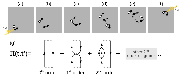
The poles and residues of the polarization propagator described by the spectral representation describe excitation energies and transition amplitudes, respectively. One possible strategy to determine these quantities is to expand $\Pi_{pq,rs}$ in a time-dependent perturbation series based on a Hamiltonian partitioned in the same way as was done for the Møller--Plesset ground-state. This expansion is also called a diagrammatic expansion because each term in the series can be represented by a Feynman diagram (see figure above). For example, the zeroth order term corresponds to non-interacting particles that propagate freely and is depicted by a diagram consisting of two parallel lines, one representing the particle (arrow pointing up) and the other representing the hole (arrow pointing down). This diagram corresponds to the situation depicted in (b) of a particle and hole propagating through the system without any further interactions. The first order term introduces direct Coulomb and exchange interactions between the particle and hole (c), while second order terms introduce interactions with a particle-hole pair generated by the initial particle and/or hole.

The above equation can be regarded as the diagonal form of the polarization propagator, which, when considering only the first term and ignoring the broadening, can be written in matrix form as

where $\boldsymbol{\Omega}$ is the diagonal matrix of excitation energies or their corresponding angular frequencies $\omega_{n0}$, and $\mathbf{x}$ are the transition amplitudes from the ground to an excited state as occurring in the numerator of the above equation, $x_{n,pq} = \bra{\Psi_n} \hat{a}_p^\dagger \hat{a}_q \ket{\Psi_0}$. Now the existence of a non-diagonal form of the polarization propagator is postulated Schirmer (1982),

where $\mathbf{M}$ is an effective interaction matrix and $\mathbf{f}$ is referred to as effective transition amplitudes. Explicit algebraic expressions for $\mathbf{M}$ and $\mathbf{f}$ are constructed by using diagrammatic perturbation theory and comparing the perturbation expansion of the original propagator (see above figure) with the perturbation expansions of the effective matrices Schirmer (1982)Dreuw & Wormit (2015) (thus explaining the perhaps odd name),

By truncating the series expansion of the polarization propagator to a desired order, different levels of ADC are obtained. The practical way to obtain the excitation energies and vectors is to assert that there is a non-diagonal matrix representation of the polarization propagator, construct this matrix, called the ADC matrix, and obtain the excitation energies and vectors via matrix diagonalization Dreuw & Wormit (2015). The ADC matrix elements can be deduced with the help of the Feynman diagrams in (g) Schirmer (1982)Wormit (2009), or via an alternative formulation of the ADC equations called the intermediate state representation (ISR), discussed in detail in the following.