Convolutional neural networks - Mathematical Modeling in Biotechnology

import numpy as np
import scipy
import sklearn

What is a convolution?¶

A convolution (or cross-correlation) combines a signal (or image) $X$ with a small kernel $K$ (also called a filter of size $k \times k$ ) by sliding the kernel across the data and computing a weighted sum at each position

(X * K)_{ij} = \sum_{m=0}^{k-1}\sum_{n=0}^{k-1} X_{i+m,\,j+n}\, K_{m,n}

(1)

For images, the kernel extracts local features such as

edges
corners
textures
simple patterns

Since the same kernel is applied everywhere, a convolutional neural network can recognize the same feature regardless of where it appears in the image. During training, the network automatically learns kernels that are useful for the prediction task.

In a fully connected neural network, every neuron in layer $L$ is connected to all neurons in layer $L-1$ through a weight matrix $\boldsymbol{W}^{(L)}$ . For image data this is wasteful: nearby pixels are related, and a pattern (an edge, a corner) can appear anywhere in the image. In contrast, a convolutional layer instead applies a small, shared set of kernel weights $\boldsymbol{K}$ that slides over the input and produces a feature map, so the number of parameters does not grow with image size and the network becomes translation invariant—a learned feature (e.g. an edge detector) is recognized wherever it occurs in the image.

Let us apply a convolution to a simple image. The argument mode controls the size of the filtered image. When set to “same” the figure size is preserved with use of padding.

image = np.zeros((20, 20))
image[5:15, 8:12] = 1

# Vertical edge detector (Sobel-x filter)
kernel = np.array([[-1, 0, 1], [-2, 0, 2], [-1, 0, 1]])

filtered = scipy.signal.correlate2d(image, kernel, mode="same")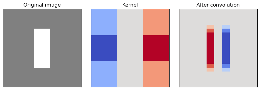

import matplotlib.pyplot as plt

fig, ax = plt.subplots(1, 3, figsize=(9, 3))

ax[0].imshow(image, cmap="gray", vmin=-1, vmax=1)
ax[0].set_title("Original image")

ax[1].imshow(kernel, cmap="coolwarm")
ax[1].set_title("Kernel")

ax[2].imshow(filtered, cmap="coolwarm")
ax[2].set_title("After convolution")

for a in ax:
    a.set_xticks([])
    a.set_yticks([])

plt.tight_layout()
plt.show()

After kernel application, the convoluted (or rather cross-correlated) image shows a positive response for a dark → white vertical edge and a negative response for a white → dark vertical edge.

To detect horizontal edges, a Sobel-y filter can be applied, which is simply the transpose of the Sobel-x filter.

Components and structure¶

A typical CNN architecture stacks a combination of the following building blocks.

Layer type	Purpose
Convolution	Extracts local features (edges, textures) using shared kernels
Activation (e.g. ReLU)	Introduces nonlinearity
Pooling	Downsamples feature maps, adding translation tolerance
Fully connected (dense)	Combines extracted features into a final prediction

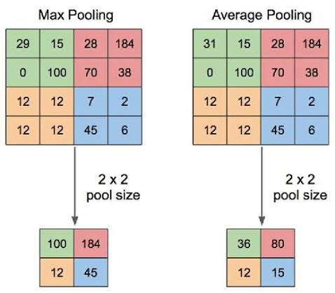
Pooling (most commonly max pooling) reduces a $p \times p$ patch of a feature map to a single value,

\mathrm{maxpool}(X)_{ij} = \max_{0 \le m,n < p} X_{ip+m,\,jp+n}

(2)

which both shrinks the data and makes the representation more robust toward small shifts in the input.

Limited-resource implementation¶

Training a full CNN (with learned kernels) usually requires a deep learning framework such as PyTorch and GPU accelerators.

On a laptop, an effective and instructive alternative is to use a small set of fixed, classical kernels (edge detectors) to perform the convolution + pooling step by hand with numpy, and then feed the resulting feature maps into a sklearn multilayer perceptron (MLP). This keeps the conceptual pipeline of a CNN (convolve → activate → pool → dense layers) while requiring minimal resources.

Data preparation¶

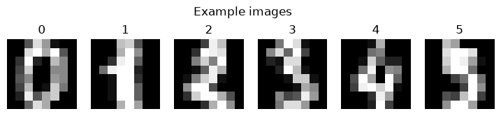
We use the digits data set: 1,797 greyscale images of handwritten digits (0-9), each $8 \times 8$ pixels.

digits = sklearn.datasets.load_digits()

X_images = digits.images  # shape (n_samples, 8, 8)
y = digits.target

print("Number of images:", X_images.shape[0])
print("Image size       :", X_images.shape[1:])

Number of images: 1797
Image size       : (8, 8)

fig, axes = plt.subplots(1, 6, figsize=(9, 2))
for ax, img, label in zip(axes, X_images[:6], y[:6]):
    ax.imshow(img, cmap="gray")
    ax.set_title(label)
    ax.axis("off")
plt.suptitle("Example images")
plt.show()

Convolution step¶

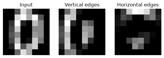
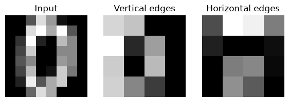
We define two small $3\times3$ kernels that act as edge detectors using horizontal and vertical Sobel filters. We apply Eq. (1) to every image and pass the result through a ReLU activation function.

sobel_x = np.array(
    [
        [-1, 0, 1],
        [-2, 0, 2],
        [-1, 0, 1],
    ]
)
sobel_y = sobel_x.T


def relu(x):
    return np.maximum(0, x)  # x can be a numpy array

def extract_features(img):

    fmap_x = relu(scipy.signal.correlate2d(img, sobel_x, mode="same"))
    fmap_y = relu(scipy.signal.correlate2d(img, sobel_y, mode="same"))

    # in return, the two 8 x 8 arrays are flattened and concatenated
    return np.concatenate([fmap_x.ravel(), fmap_y.ravel()])


X_features = np.array([extract_features(img) for img in X_images])

print("Image feature vector length:", X_features.shape[1])

Image feature vector length: 128

example = X_images[0]

fmap_x = relu(scipy.signal.correlate2d(example, sobel_x, mode="same"))
fmap_y = relu(scipy.signal.correlate2d(example, sobel_y, mode="same"))

fig, axes = plt.subplots(1, 3, figsize=(7, 2.5))

axes[0].imshow(example, cmap="gray")
axes[0].set_title("Input")

axes[1].imshow(fmap_x, cmap="gray")
axes[1].set_title("Vertical edges")

axes[2].imshow(fmap_y, cmap="gray")
axes[2].set_title("Horizontal edges")

for ax in axes:
    ax.axis("off")

plt.show()

Pooling step¶

On top of the convolution and the activation we then apply $2\times2$ max pooling, Eq. (2).

def maxpool2d(img, p=2):
    h, w = img.shape

    # Divide the image into non-overlapping p x p regions and replace
    # each region by its largest value (max pooling).
    return img.reshape(h // p, p, w // p, p).max(axis=(1, 3))


def extract_features(img):

    fmap_x = maxpool2d(relu(scipy.signal.correlate2d(img, sobel_x, mode="same")))
    fmap_y = maxpool2d(relu(scipy.signal.correlate2d(img, sobel_y, mode="same")))

    # in return, the two 4 x 4 arrays are flattened and concatenated
    return np.concatenate([fmap_x.ravel(), fmap_y.ravel()])


X_features = np.array([extract_features(img) for img in X_images])

print("Image feature vector length:", X_features.shape[1])

Image feature vector length: 32

example = X_images[0]

fmap_x = maxpool2d(relu(scipy.signal.correlate2d(example, sobel_x, mode="same")))
fmap_y = maxpool2d(relu(scipy.signal.correlate2d(example, sobel_y, mode="same")))

fig, axes = plt.subplots(1, 3, figsize=(7, 2.5))

axes[0].imshow(example, cmap="gray")
axes[0].set_title("Input")

axes[1].imshow(fmap_x, cmap="gray")
axes[1].set_title("Vertical edges")

axes[2].imshow(fmap_y, cmap="gray")
axes[2].set_title("Horizontal edges")

for ax in axes:
    ax.axis("off")

plt.show()

Split and scale data¶

X_train, X_test, y_train, y_test = sklearn.model_selection.train_test_split(
    X_features,
    y,
    test_size=0.20,
    stratify=y,
)

scaler = sklearn.preprocessing.StandardScaler()
X_train_scaled = scaler.fit_transform(X_train)
X_test_scaled = scaler.transform(X_test)

Dense (fully connected) classifier head¶

The pooled feature maps have been flattened and are fed into an MLPClassifier, exactly as in the basic neural network notebook.

This plays the role of the fully connected layers at the end of a CNN.

mlp = sklearn.neural_network.MLPClassifier(
    hidden_layer_sizes=(32, 32),
    activation="relu",
    solver="adam",
    max_iter=500,
)

mlp.fit(X_train_scaled, y_train)

Model evaluation¶

y_pred = mlp.predict(X_test_scaled)

print(sklearn.metrics.classification_report(y_test, y_pred))

              precision    recall  f1-score   support

           0       1.00      1.00      1.00        36
           1       0.97      0.97      0.97        37
           2       0.95      1.00      0.97        35
           3       0.97      0.97      0.97        37
           4       1.00      0.92      0.96        36
           5       0.97      0.94      0.96        36
           6       1.00      1.00      1.00        36
           7       0.97      1.00      0.99        36
           8       0.89      0.97      0.93        35
           9       0.97      0.92      0.94        36

    accuracy                           0.97       360
   macro avg       0.97      0.97      0.97       360
weighted avg       0.97      0.97      0.97       360

cm = sklearn.metrics.confusion_matrix(y_test, y_pred)
disp = sklearn.metrics.ConfusionMatrixDisplay(confusion_matrix=cm)
disp.plot(cmap=plt.cm.Blues)
plt.title("CNN-style pipeline: confusion matrix")
plt.show()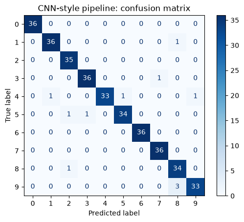

Remarks¶

Using ReLu discards all of the negative responses and even with another activation function, max pooling would discard them in the pooling step.
This is still done in practice rather than using e.g. tanh and an adapted pooling strategy, because they are much faster to compute.
The lack of negative response information is in practice compensated for by using a second filter per dimension, which gives the same responses with opposite signs.

Take-away¶

General¶

A real CNN learns the kernels (rather than using fixed Sobel filters) through backpropagation, and stacks many convolution/pooling blocks.
The pipeline above including convolve, activate, pool, flatten, and dense is exactly the structure of a CNN, and our reproducing it with fixed kernels and sklearn is a lightweight way to build intuition before moving to a full deep learning framework (e.g. PyTorch torch.nn.Conv2d) for projects that need learned filters and larger image data sets.

Bioengineering applications¶

Convolutional neural networks are widely used for image-based biological and medical data, for example microscopy images of cells, histopathology slides, fluorescence microscopy and radiological images.

In this course we avoid additional deep-learning dependencies and instead use a numpy/scipy/sklearn style implementation to illustrate the underlying computations. In practice, these models are almost always implemented using PyTorch or TensorFlow/Keras.

Model selection¶

As for all supervised learning methods, hyperparameters (number of filters, kernel size, pooling strategy, learning rate and network depth) should be selected using a validation set or cross-validation rather than the test set. Typical scikit-learn tools are train_test_split, cross_val_score, GridSearchCV and RandomizedSearchCV.