Graph neural networks - Mathematical Modeling in Biotechnology

import networkx as nx
import numpy as np
import sklearn

Why graphs?¶

Many data sets are naturally structured as a graph $G = (V, E)$ of nodes (or vertices) $V$ connected by edges $E$ , rather than as a table of independent feature vectors.

This is highly relevant in biology and chemistry. E.g. molecules can be represented as graphs of atoms (nodes) connected by bonds (edges), and the same topology-based representation applies to protein–protein interaction networks, metabolic networks, and knowledge graphs in biomedicine.

A graph neural network (GNN) learns node representations that take this connectivity into account, by repeatedly mixing each node’s features with those of its neighbors.

Typical prediction tasks include:

Node classification: Predict properties of individual nodes, such as the function of a protein in a protein–protein interaction network or the community of a person in a social network.
Link prediction: Predict whether two nodes should be connected, for example whether two proteins interact or whether a drug is likely to bind to a molecular target.
Graph classification: Predict properties of an entire graph. In biotechnology, this often means predicting molecular properties such as toxicity, solubility, biological activity, or drug-likeness from a molecular structure.
Graph regression: Predict a continuous quantity associated with a graph, such as binding affinity, reaction yield, or a physicochemical property of a molecule.

Components and structure¶

In a standard MLP, each neuron produces a single scalar activation value. In contrast, each node in a GNN is associated with a feature vector whose components are updated through message passing. We denote the feature vector of node $n$ in layer $L$ as $\boldsymbol{h}_n^{(L)}$ .

Moreover, instead of a single dense weight matrix connecting all neurons of one layer to the next, a GNN layer only mixes a node’s features with those of its graph neighbors $\mathcal{N}(n)$ :

\mathbf{h}_n^{(L)} = f \left( \mathbf{h}_n^{(L-1)}, \left\{ \mathbf{h}_k^{(L-1)} : k \in \mathcal{N}(n) \right\} \right)

(1)

The graph connectivity is stored in the adjacency matrix $\boldsymbol{A}$ ( $A_{ij}=1$ if nodes $i$ and $j$ are connected) and the degree matrix $\boldsymbol{D}$ (diagonal, $D_{ii}$ = number of neighbors of node $i$ ).

Collecting all node feature vectors as rows of a matrix $\boldsymbol{H}$ allows the message-passing operation to be written compactly in matrix form. The graph convolutional network (GCN) is a widely used form of GNN for which layer propagation reads

\boldsymbol{H}^{(L)} = f\!\left( \tilde{\boldsymbol{D}}^{-1/2} \tilde{\boldsymbol{A}} \, \tilde{\boldsymbol{D}}^{-1/2} \, \boldsymbol{H}^{(L-1)} \boldsymbol{W}^{(L)} \right)

(2)

where $\tilde{\boldsymbol{A}} = \boldsymbol{A} + \boldsymbol{I}$ adds a self-loop to every node (so a node also retains its own information), $\tilde{\boldsymbol{D}}$ is the corresponding degree matrix, $\boldsymbol{W}^{(L)}$ is a (shared, learnable) weight matrix, and $f$ is a nonlinear activation function.

You can think of this as $\boldsymbol{A}_\mathrm{norm} = \tilde{\boldsymbol{D}}^{-1/2} \tilde{\boldsymbol{A}} \tilde{\boldsymbol{D}}^{-1/2}$ representing a kernel, leading to a similar convolution or rather cross-correlation layer as already seen in the CNN notebook. Stacking $K$ such layers lets information flow $K$ hops away from each node — this is known as message passing.

Training the weight matrices¶

The weight matrices $\boldsymbol{W}^{(L)}$ are learned by minimizing a loss function with gradient descent, exactly as in the basic neural network notebook. For binary node classification with labels $y_i \in \{0,1\}$ we use the averaged binary cross-entropy loss restricted to the training nodes

\mathcal{L} = - \frac{1}{N_\mathcal{T}} \sum_{i \in \mathcal{T}} \Big[ y_i \log \hat{y}_i + (1-y_i)\log(1-\hat{y}_i) \Big]

(3)

where $N_\mathcal{T}$ is the number of training nodes.

Because $\boldsymbol{A}_\mathrm{norm}$ is fixed and symmetric, backpropagating through each GCN layer (Eq. (2)) simply involves multiplying the incoming gradient by $\boldsymbol{A}_\mathrm{norm}$ and $\boldsymbol{W}^{(L)\top}$ — exactly as for an ordinary dense layer, with one extra fixed matrix multiplication.

Node classification example¶

Data preparation¶

We will use Zachary’s karate club graph as an illustration of node classification. It contains 34 featureless nodes (club members) of a university karate club together with 78 edges (friendships among members). After a conflict, the club split into two factions representing the node classes that we will predict from the graph structure and connectivity patterns.

This is a standard toy benchmark for GNNs, and the problem is entirely analogous to classifying nodes in any small biological network where community membership is the target (e.g. assigning proteins to functional modules in an interaction network).

G = nx.karate_club_graph()

n_nodes = G.number_of_nodes()
nodes = list(G.nodes())

# create target data: "0" for club "Mr. Hi" and "1" for club "Officer"
y = np.array([0 if G.nodes[n]["club"] == "Mr. Hi" else 1 for n in nodes])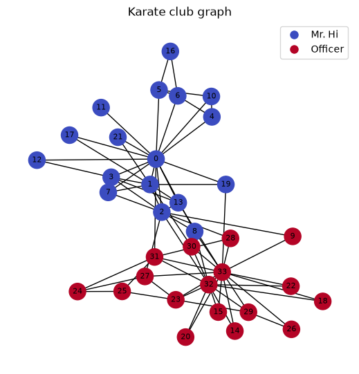

import matplotlib.pyplot as plt

plt.figure(figsize=(5, 5))

pos = nx.spring_layout(G, seed=0)

nx.draw(
    G,
    pos,
    node_color=y,
    cmap=plt.cm.coolwarm,
    with_labels=True,
    node_size=300,
    font_size=8,
)

from matplotlib.lines import Line2D

legend_elements = [
    Line2D(
        [0],
        [0],
        marker="o",
        color="w",
        label="Mr. Hi",
        markerfacecolor=plt.cm.coolwarm(0.0),
        markersize=10,
    ),
    Line2D(
        [0],
        [0],
        marker="o",
        color="w",
        label="Officer",
        markerfacecolor=plt.cm.coolwarm(1.0),
        markersize=10,
    ),
]

plt.legend(handles=legend_elements)

plt.title("Karate club graph")

plt.show()

Initial node features and graph normalization¶

The Karate Club graph is effectively featureless in terms of meaningful node attributes, but we initialize nodes with one-hot identifiers so that the GCN can distinguish between them.

In practice, this means that we choose to set feature matrix $\boldsymbol{H}^{(0)}$ equal to the $N \times N$ identity matrix.

The propagation rule of Eq. (2) then turns pure structural connectivity into informative lower-dimensional embeddings.

H0 = np.identity(n_nodes, dtype=float)

Since it does not change during training, we pre-compute the normalized adjacency matrix $\boldsymbol{A}_\mathrm{norm}$ .

A = nx.to_numpy_array(G)
A_tilde = A + np.identity(n_nodes, dtype=float)

D_inv_sqrt = np.diag(1.0 / np.sqrt(A_tilde.sum(axis=1)))

A_norm = D_inv_sqrt @ A_tilde @ D_inv_sqrt

Train / test split¶

We split the nodes into training and test sets and use the stratify argument to maintain equal proportion of node classes in the two sets.

train_idx, test_idx = sklearn.model_selection.train_test_split(
    np.arange(n_nodes),
    test_size=0.25,
    stratify=y,
    random_state=0,
)

train_mask = np.zeros(n_nodes, dtype=bool)
train_mask[train_idx] = True

Model definition¶

We implement a two-layer GCN:

two propagation layers (Eq. (2)) with ReLU activations
one linear readout layer with a sigmoid to produce node-level class probabilities

def relu(x):
    return np.maximum(0.0, x)


def relu_grad(x):
    return (x > 0.0).astype(float)


def sigmoid(x):
    return 1.0 / (1.0 + np.exp(-x))

The learnable weight matrices are randomly initialized, while the bias in the readout layer is initialized to zero.

def init_weights(fan_in, fan_out, rng):
    return rng.normal(scale=np.sqrt(2.0 / fan_in), size=(fan_in, fan_out))


rng_w = np.random.default_rng(0)
W1 = init_weights(n_nodes, 8, rng_w)
W2 = init_weights(8, 4, rng_w)
W3 = init_weights(4, 1, rng_w)

b3 = np.zeros(1)

We implement forward propagation in the network. The forward propagation consists of a sequence of message-passing layers, followed by a readout (pooling) step and a prediction layer.

def forward(H0):

    Z1 = A_norm @ H0 @ W1
    H1 = relu(Z1)  # shape (N, 8)

    Z2 = A_norm @ H1 @ W2
    H2 = relu(Z2)  # shape (N, 4)

    logits = H2 @ W3 + b3  # shape (N, 1)

    y_hat = sigmoid(logits).ravel()

    return y_hat, (H0, Z1, H1, Z2, H2)

The gradient of the loss function is obtained with the standard technique of backpropagation.

def backward(y_true, y_hat, cache, mask):

    H0, Z1, H1, Z2, H2 = cache

    n_train = mask.sum()

    # gradient of cross-entropy loss w.r.t. logits, zeroed for test nodes
    dlogits = np.zeros((n_nodes, 1))
    dlogits[mask, 0] = (y_hat[mask] - y_true[mask]) / n_train

    # readout layer
    dW3 = H2.T @ dlogits
    db3 = dlogits.sum(axis=0)

    # layer 2: Z2 = A_norm @ H1 @ W2
    dH2 = dlogits @ W3.T
    dZ2 = dH2 * relu_grad(Z2)
    dW2 = (A_norm @ H1).T @ dZ2
    dH1 = A_norm @ dZ2 @ W2.T  # A_norm is symmetric

    # layer 1: Z1 = A_norm @ H0 @ W1
    dZ1 = dH1 * relu_grad(Z1)
    dW1 = (A_norm @ H0).T @ dZ1

    return dW1, dW2, dW3, db3

Model training¶

We minimize the loss function with respect to weight and bias parameters using the gradient descent method.

lr = 0.5  # learning rate, or step length
n_epochs = 500
losses = []
eps = 1e-9

for epoch in range(n_epochs):

    y_hat, cache = forward(H0)

    loss = -np.mean(
        y[train_mask] * np.log(y_hat[train_mask] + eps)
        + (1 - y[train_mask]) * np.log(1 - y_hat[train_mask] + eps)
    )
    losses.append(loss)

    dW1, dW2, dW3, db3_ = backward(y, y_hat, cache, train_mask)
    W1 -= lr * dW1
    W2 -= lr * dW2
    W3 -= lr * dW3
    b3 -= lr * db3_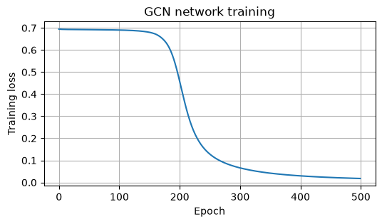

Model evaluation¶

We evaluate the model by its predictions for the classification of the test nodes.

y_hat_final, _ = forward(H0)
y_pred = (y_hat_final > 0.5).astype(int)

print(
    sklearn.metrics.classification_report(
        y[test_idx],  # ground truth
        y_pred[test_idx],  # model predictions
        target_names=["Mr. Hi", "Officer"],
    )
)

              precision    recall  f1-score   support

      Mr. Hi       1.00      1.00      1.00         5
     Officer       1.00      1.00      1.00         4

    accuracy                           1.00         9
   macro avg       1.00      1.00      1.00         9
weighted avg       1.00      1.00      1.00         9

cm = sklearn.metrics.confusion_matrix(y[test_idx], y_pred[test_idx])

disp = sklearn.metrics.ConfusionMatrixDisplay(
    confusion_matrix=cm, display_labels=["Mr. Hi", "Officer"]
)
disp.plot(cmap=plt.cm.Blues)

plt.title("Confusion matrix")

plt.show()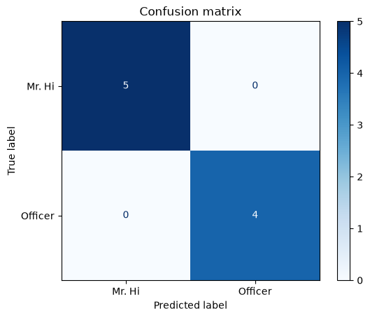

We note that all test nodes are correctly classified based on their graph connectivity patterns.

Remarks¶

The learning rate, number of epochs, and hidden layer sizes above were fixed by hand. As discussed in more detail in the CNN notebook, these should be tuned by cross-validation. For a hand-written training loop sklearn.model_selection.KFold can still generate the node-index splits for each fold, even though the gradient descent loop is custom coded.
The Karate Club graph is extremely small and should not be viewed as a realistic benchmark. In practice, graph prediction problems are substantially more difficult.

Take-away¶

Implementation¶

In this notebook the weight matrices $\boldsymbol{W}^{(L)}$ in Eq. (2) were learned by gradient descent written out by hand — the same principle as the basic neural network notebook, with one extra multiplication by the fixed $\boldsymbol{A}_\mathrm{norm}$ at every layer.
For real-world graphs, arising from e.g. molecules with atom and bond features or large protein interaction networks, dedicated libraries are needed.
PyTorch Geometric and DGL provide optimized, GPU-accelerated GCN layers with routines for differentiation and mini-batching over large graphs.
scikit-network is a lighter-weight alternative for fast classical graph algorithms (community detection, spectral embeddings, centrality) within the sklearn-style API, though it does not provide trainable GNN layers.

Message passing interpretation¶

One GCN layer allows a node to gather information from its direct neighbors.

After:

one layer: 1-hop neighborhood
two layers: 2-hop neighborhood
three layers: 3-hop neighborhood

Thus, increasing the number of GCN layers increases the portion of the graph that can influence a node.

Features¶

The Karate Club graph does not contain meaningful node attributes such as age, income, or protein expression levels. To allow the GCN to distinguish between nodes, each node is initialized with a one-hot feature vector (the rows of the identity matrix). The model must therefore learn almost entirely from the graph structure itself.
In molecular applications, the initial node features would instead contain chemically meaningful quantities such as atomic number, formal charge, or aromaticity. More advanced molecular GNNs may also use edge features to represent bond types.