Gradient boosting - Mathematical Modeling in Biotechnology

Why ensembles?¶

A single decision tree tends to overfit: it has high variance, meaning small changes in the training data can produce a very different tree. Ensemble methods combine many trees to produce predictions that are more accurate and more stable than any individual tree. Gradient boosting is the classic boosting strategy; the other major strategy is bagging (random forests).

Gradient boosting¶

Gradient boosting builds trees sequentially, where each new tree is trained to correct the errors (residuals) of the ensemble built so far. The ensemble after $m$ trees is

F_m(\boldsymbol{x}) = F_{m-1}(\boldsymbol{x}) + \eta \, h_m(\boldsymbol{x})

(1)

where $h_m$ is a new, typically shallow tree fitted to the negative gradient of the loss function with respect to $F_{m-1}$ (the residuals, in the case of squared-error loss), and $\eta$ is a small learning rate that controls how much each new tree is allowed to contribute. Unlike bagging, boosting reduces bias: individual trees are deliberately kept weak (shallow), and the ensemble gradually becomes more expressive as trees are added — which also means that, unlike a random forest, adding too many trees can eventually overfit.

Library imports¶

import matplotlib.pyplot as plt
import sklearn

Data preparation¶

We reuse the breast cancer data set from the decision tree notebook.

cancer = sklearn.datasets.load_breast_cancer()
X, y = cancer["data"], cancer["target"]

X_train, X_test, y_train, y_test = sklearn.model_selection.train_test_split(
    X, y, test_size=0.20, stratify=y, random_state=0,
)

Model definition and training¶

We build a sequential ensemble of 200 shallow trees, Eq. (1), each trained to correct the remaining errors, with a small learning rate $\eta$ .

gb = sklearn.ensemble.GradientBoostingClassifier(
    n_estimators=200,
    max_depth=2,
    learning_rate=0.1,
    random_state=0,
)

gb.fit(X_train, y_train)

y_pred_gb = gb.predict(X_test)
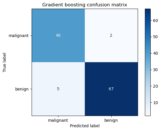
print(sklearn.metrics.classification_report(y_test, y_pred_gb, target_names=cancer["target_names"]))

              precision    recall  f1-score   support

   malignant       0.89      0.95      0.92        42
      benign       0.97      0.93      0.95        72

    accuracy                           0.94       114
   macro avg       0.93      0.94      0.93       114
weighted avg       0.94      0.94      0.94       114

Effect of ensemble size: staged predictions¶

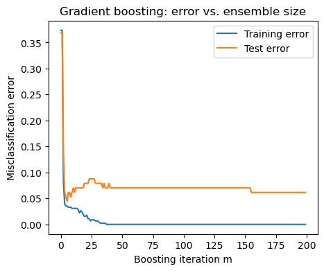
Because boosting adds trees sequentially, sklearn lets us inspect the ensemble’s error after every stage using staged_predict, without refitting. This shows both the bias-reducing benefit of adding trees and the overfitting risk mentioned above: training error keeps dropping, while test error eventually flattens (and can even start creeping up) as more trees are added.

train_errors, test_errors = [], []

for y_pred_train, y_pred_test in zip(gb.staged_predict(X_train), gb.staged_predict(X_test)):
    train_errors.append(1 - sklearn.metrics.accuracy_score(y_train, y_pred_train))
    test_errors.append(1 - sklearn.metrics.accuracy_score(y_test, y_pred_test))

plt.figure(figsize=(5, 4))
plt.plot(train_errors, label="Training error")
plt.plot(test_errors, label="Test error")
plt.xlabel("Boosting iteration m")
plt.ylabel("Misclassification error")
plt.title("Gradient boosting: error vs. ensemble size")
plt.legend()
plt.show()

Comparing a single tree to gradient boosting¶

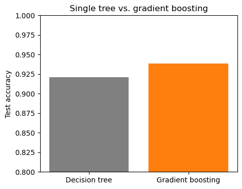
To highlight the effect of boosting, we also fit a single decision tree of comparable depth and compare test accuracy.

tree = sklearn.tree.DecisionTreeClassifier(max_depth=3, random_state=0)
tree.fit(X_train, y_train)

models = {
    "Decision tree": tree,
    "Gradient boosting": gb,
}
accuracies = {name: sklearn.metrics.accuracy_score(y_test, m.predict(X_test)) for name, m in models.items()}

plt.figure(figsize=(5, 4))
plt.bar(accuracies.keys(), accuracies.values(), color=["gray", "tab:orange"])
plt.ylabel("Test accuracy")
plt.ylim(0.8, 1.0)
plt.title("Single tree vs. gradient boosting")
plt.show()

Model evaluation¶

cm = sklearn.metrics.confusion_matrix(y_test, y_pred_gb)
disp = sklearn.metrics.ConfusionMatrixDisplay(confusion_matrix=cm, display_labels=cancer["target_names"])
disp.plot(cmap=plt.cm.Blues)
plt.title("Gradient boosting confusion matrix")
plt.show()

Feature importance¶

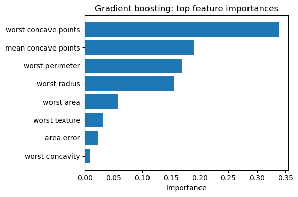
As with a single tree, the ensemble provides an aggregated feature importance, averaged over all 200 trees.

importances = gb.feature_importances_
order = importances.argsort()[::-1][:8]

plt.figure(figsize=(6, 4))
plt.barh(
    [cancer["feature_names"][i] for i in order][::-1],
    importances[order][::-1],
)
plt.xlabel("Importance")
plt.title("Gradient boosting: top feature importances")
plt.tight_layout()
plt.show()

Take-away¶

Gradient boosting (and optimized implementations such as XGBoost or LightGBM) tends to achieve the best raw predictive performance on tabular data among tree-based methods, at the cost of more careful tuning of n_estimators, max_depth, and learning_rate to avoid overfitting — unlike a random forest, simply adding more trees is not always safe. In practice it is common to start with a random forest as a robust baseline and move to gradient boosting once there is time and validation data available to tune it properly.