Random forests - Mathematical Modeling in Biotechnology

Why ensembles?¶

A single decision tree tends to overfit: it has high variance, meaning small changes in the training data can produce a very different tree. Ensemble methods combine many trees to produce predictions that are more accurate and more stable than any individual tree. Random forests are the classic bagging strategy; the other major strategy is boosting (gradient boosting).

Random forests (bagging)¶

A random forest builds $M$ decision trees independently and in parallel, each on a bootstrap sample (random sample with replacement) of the training data, and additionally restricts each split to a random subset of features. Predictions are then averaged (regression) or majority-voted (classification) across all trees,

\hat{y} = \frac{1}{M} \sum_{m=1}^{M} T_m(\boldsymbol{x})

(1)

where $T_m$ denotes the prediction of the $m$ -th tree. Averaging many noisy, independently trained, mostly-uncorrelated trees reduces the overall variance without increasing bias — individual trees can be deep and somewhat overfit, since their errors tend to cancel out in the average. This is why random forests reduce variance rather than bias: unlike boosting, adding more trees essentially never hurts.

Library imports¶

import matplotlib.pyplot as plt
import sklearn

Data preparation¶

We reuse the breast cancer data set from the decision tree notebook.

cancer = sklearn.datasets.load_breast_cancer()
X, y = cancer["data"], cancer["target"]

X_train, X_test, y_train, y_test = sklearn.model_selection.train_test_split(
    X, y, test_size=0.20, stratify=y, random_state=0,
)

Model definition and training¶

We build a forest of 200 trees, Eq. (1), each trained on a bootstrap sample with a random subset of features considered at every split.

rf = sklearn.ensemble.RandomForestClassifier(
    n_estimators=200,
    max_depth=None,
    random_state=0,
)

rf.fit(X_train, y_train)

y_pred_rf = rf.predict(X_test)
print(sklearn.metrics.classification_report(y_test, y_pred_rf, target_names=cancer["target_names"]))

              precision    recall  f1-score   support

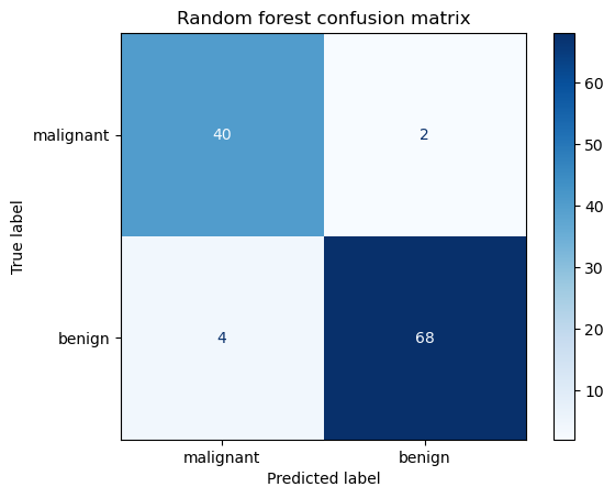
   malignant       0.91      0.95      0.93        42
      benign       0.97      0.94      0.96        72

    accuracy                           0.95       114
   macro avg       0.94      0.95      0.94       114
weighted avg       0.95      0.95      0.95       114

Effect of ensemble size: out-of-bag error¶

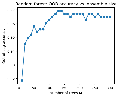
Because each tree only sees a bootstrap sample (roughly 63% of the training set), the remaining out-of-bag (OOB) samples can be used as a free internal validation set, without touching the held-out test set. We track the OOB accuracy as trees are added, illustrating that bagging error decreases and then plateaus — it does not go back up as $M$ grows, which is the practical signature of variance reduction.

n_estimators_range = range(10, 301, 10)
oob_scores = []

for n in n_estimators_range:
    rf_oob = sklearn.ensemble.RandomForestClassifier(
        n_estimators=n, max_depth=None, oob_score=True, random_state=0,
    )
    rf_oob.fit(X_train, y_train)
    oob_scores.append(rf_oob.oob_score_)

plt.figure(figsize=(5, 4))
plt.plot(list(n_estimators_range), oob_scores, "o-")
plt.xlabel("Number of trees M")
plt.ylabel("Out-of-bag accuracy")
plt.title("Random forest: OOB accuracy vs. ensemble size")
plt.show()

Comparing a single tree to the random forest¶

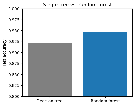
To highlight the effect of bagging, we also fit a single decision tree of comparable depth and compare test accuracy.

tree = sklearn.tree.DecisionTreeClassifier(max_depth=3, random_state=0)
tree.fit(X_train, y_train)

models = {
    "Decision tree": tree,
    "Random forest": rf,
}
accuracies = {name: sklearn.metrics.accuracy_score(y_test, m.predict(X_test)) for name, m in models.items()}

plt.figure(figsize=(5, 4))
plt.bar(accuracies.keys(), accuracies.values(), color=["gray", "tab:blue"])
plt.ylabel("Test accuracy")
plt.ylim(0.8, 1.0)
plt.title("Single tree vs. random forest")
plt.show()

Model evaluation¶

cm = sklearn.metrics.confusion_matrix(y_test, y_pred_rf)
disp = sklearn.metrics.ConfusionMatrixDisplay(confusion_matrix=cm, display_labels=cancer["target_names"])
disp.plot(cmap=plt.cm.Blues)
plt.title("Random forest confusion matrix")
plt.show()

Feature importance¶

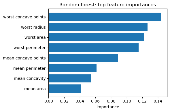
As with a single tree, the forest provides an aggregated feature importance, averaged over all 200 trees.

importances = rf.feature_importances_
order = importances.argsort()[::-1][:8]

plt.figure(figsize=(6, 4))
plt.barh(
    [cancer["feature_names"][i] for i in order][::-1],
    importances[order][::-1],
)
plt.xlabel("Importance")
plt.title("Random forest: top feature importances")
plt.tight_layout()
plt.show()

Take-away¶

Random forests are an excellent default choice for tabular data with limited resources: they require little preprocessing (no feature scaling), handle a mix of numerical and categorical features well, and are robust to hyperparameter choices — they rarely need extensive tuning, and adding more trees essentially never hurts. Their main weakness relative to boosting (companion notebook) is that they typically leave a bit of predictive performance on the table, since averaging independent trees reduces variance but does nothing to reduce bias.