Scipy for ODEs - Mathematical Modeling in Biotechnology

Differential equations¶

An equation relating one or more functions (or state variables) and their derivatives is known as a differential equation. They play a prominent role in natural sciences and engineering as exemplified by the heat equation

\frac{\partial u}{\partial t} = \alpha \Big( \frac{\partial^2 u}{\partial x^2} + \frac{\partial^2 u}{\partial y^2} + \frac{\partial^2 u}{\partial z^2} \Big)

(1)

where $u(x,y,z,t)$ is the temperature at point $\mathbf{r} = (x,y,z)$ at time $t$ and $\alpha$ is a positive constant known as the thermal diffusivity of the medium.

Finite difference method (FDM)¶

Numerical solutions are obtained by discretizing the functions in space and time and approximating derivatives with finite differences, e.g.,

\frac{\partial u}{\partial t} \approx \frac{u(t + \Delta t) - u(t)}{\Delta t}

(2)

and

\begin{align*} \frac{\partial^2 u}{\partial x^2} & \approx \Big( \frac{u(x + \Delta x) - u(x)}{\Delta x} - \frac{u(x) - u(x - \Delta x)}{\Delta x} \Big) / \Delta x \\ & = \frac{u(x + \Delta x) - 2 u(x) + u(x - \Delta x)}{(\Delta x)^2} \end{align*}

(3)

Providing initial values for the functions allows us to propogate the differential equation.

Model heat transfer through a wall¶

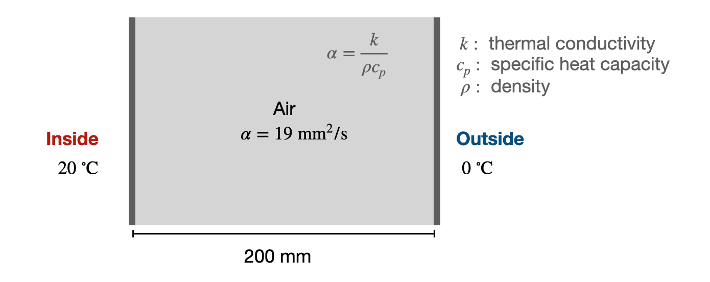
Figure 1:Heat transfer through a wall as an example of solving the heat equation in 1D.

We write a class for a wall with heat transfer that stores the state variable $u(x)$ and contains a method to conduct an Euler step in the time propagation.

import numpy as np


class HeatTransferWall:
    def __init__(self, thickness, T_inside, T_outside, alpha=19, N=100):

        self.alpha = alpha  # diffusivity with default value for air
        self.number_elements = N
        self.dx = thickness / N

        # initialization of state variable u(x)
        self.x = np.linspace(0, thickness, N)
        self.u = np.ones(N) * T_outside
        self.u[0] = T_inside

    def step(self, dt=0.1):

        N = self.number_elements

        d2u_dx2 = np.zeros(N)
        d2u_dx2[1 : N - 1] = (
            self.u[2:N] - 2 * self.u[1 : N - 1] + self.u[0 : N - 2]
        ) / self.dx**2
        # Euler step
        self.u[1 : N - 1] = self.u[1 : N - 1] + self.alpha * d2u_dx2[1 : N - 1] * dt

Propagate the heat equation for 5 min in time steps of 0.1 sec.

wall = HeatTransferWall(200, 20, 0)

for i in range(3000):
    wall.step()

Plot the final state, $u(x, T)$ .

import matplotlib.pyplot as plt

fig = plt.figure(figsize=(8, 4))

plt.plot(wall.x, wall.u)

plt.grid("on")
plt.ylabel(r"Temperature ($^\circ$C)")
plt.xlabel("Wall position (mm)")

plt.show()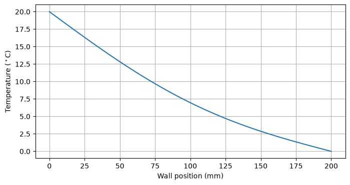

In this implementation, we did not save the intermediate states, $u(x,t)$ for $0 \leq t \leq T$ , but it is of course straighforward to do so.

# enable an interactive plot
%matplotlib notebook

import numpy as np
import matplotlib.pyplot as plt
from matplotlib.animation import FuncAnimation

wall = HeatTransferWall(200, 20, 0)

fig = plt.figure(figsize = (8,4))
ax = plt.axes(xlim=(0, 200), ylim=(-1, 21))
ax.grid()

plt.ylabel(r'Temperature ($^\circ$C)')
plt.xlabel('Wall position (mm)')

# create line and text objects
line, = ax.plot(wall.x, wall.u, lw=2)
time_text = ax.text(130, 19, 'Time: 0 (sec)')

def plot_update(frame_number, wall, line, time_text):

    # perform a time step
    wall.step()
    
    # update properties of line and text objects
    line.set_data(wall.x, wall.u)
    time_text.set_text(f'Time: {frame_number} (sec)')

# run the animation
anim = FuncAnimation(fig, plot_update, fargs = [wall, line, time_text], frames = 3000, interval = 2)

plt.show()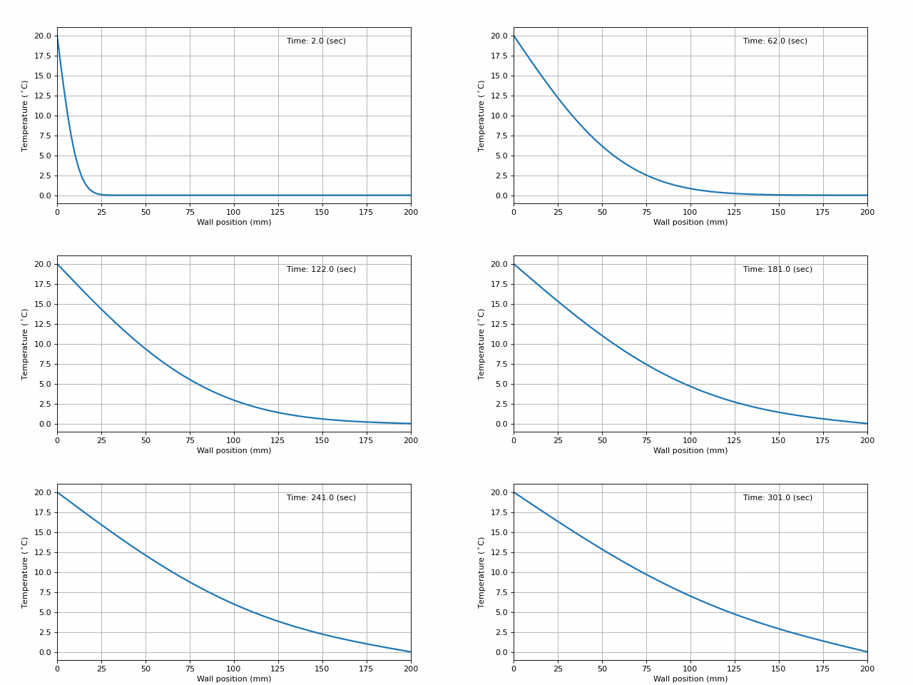

Figure 2:Animation of heat transfer through a wall.

Ordinary differential equations (ODEs)¶

Implicit form¶

In describing the dynamics of biological system, we are typically concerned with ordinary differential equations (ODEs) in which case the state variables are functions of time only and partial derivatives are replaced by “ordinary” derivatives. A system of implicit ODEs may be quite generally written

\mathbf{F}(\mathbf{y}', \mathbf{y}, t) = 0

(4)

where $\mathbf{y}$ is the array collecting the set of state variables, $\mathbf{y}'$ denotes its time derivative, and $\mathbf{F}$ is the array collecting the set of scalar equations.

It may at first sight appear limiting not to consider higher-order derivatives of $\mathbf{y}$ , such as the second-order derivative $\mathbf{y}''$ , as arguments of $\mathbf{F}$ . However, an ODE of order greater than one can be re-written as a system of ODEs of first order. As an illustration, let us consider the second-order differential equation describing the Newtonian mechanics of a damped harmonic oscillator

m \frac{d^2 x}{d t^2} = -c \frac{d x}{d t} - k x

(5)

where $k$ is the spring constant and the friction, or damping, is proportional to the velocity of the particle. Let us introduce

\begin{align*} y_1 & = x \\ y_2 & = x' \end{align*}

(6)

which transforms the one-dimensional second-order differential equation into a two-dimensional first-order differential equation according to

\begin{align*} y_1' & = y_2 \\ y_2' & = -\frac{c}{m} y_2 - \frac{k}{m} y_1 \end{align*}

(7)

Explicit form¶

Less general than the implicit case, an explicit system of ODE takes the form

\mathbf{y}' = \mathbf{F}(\mathbf{y}, t)

(8)

where it is thus required that the equations are linear in $\mathbf{y}'$ .

The Lotka–Volterra (or predator–prey) equations represents an example of an explicit system of ODEs.

\begin{align*} \frac{dy_1}{dt} & = \alpha y_1 - \beta y_1 y_2 \qquad \mathsf{(Prey)}\\ \frac{dy_2}{dt} & = \delta y_1 y_2 - \gamma y_2 \qquad \mathsf{(Predator)} \end{align*}

(9)

where $\mathbf{y} = (y_1, y_2)$ .

Model design¶

Designing a model to describe a real-world situation refers to the introduction of a canonical set of state variables, their couplings and parameters, and relating the parameters to actual conditions.

E.g. we may wish to embed the following facts into the model:

Prey has one offspring per year, i.e., $\alpha = \mathrm{ln}(2)$
Predator has at most one offspring per year but fewer when prey is short, i.e., $\delta y_1 = \min(\mathrm{ln}(2), \delta y_1)$

Numerical solutions¶

Euler’s method¶

Knowledge of the state variables collected in $\mathbf{y}$ at some time $t_0$ makes it straightforward to find a numerical solution to an explicit system of ODEs. We discretize time and use a differential approximation of the derivative according to

\mathbf{y}(t + \Delta t) = \mathbf{y}(t) + \mathbf{F}(\mathbf{y}, t) \Delta t

(10)

This approach is called the Euler method and we shall illustrate its use by finding a solution to the Lotka–Volterra equations. In doing so, we will also take the opportunity to illustrate that Python naturally invites to good software engineering practices in terms of object-oriented programming.

class PredatorPreyModel:
    def __init__(self, y0, alpha, beta, delta, gamma):
        """
        Model parameters:
        =================
        y0: initial (predator, prey) populations

        alpha: prey growth rate
        beta: prey death rate
        delta: predator growth rate
        gamma: predator death rate
        """
        self.alpha = alpha
        self.beta = beta
        self.gamma = gamma
        self.delta = delta

        self.preys = [y0[0]]
        self.predators = [y0[1]]

    def euler_step(self, dt):

        y1 = self.preys[-1]
        y2 = self.predators[-1]

        delta = self.delta
        if delta * y1 > np.log(2):
            delta = np.log(2) / y1

        y1_new = y1 + (self.alpha * y1 - self.beta * y1 * y2) * dt
        y2_new = y2 + (delta * y1 * y2 - self.gamma * y2) * dt

        self.preys.append(y1_new)
        self.predators.append(y2_new)

First, we discretize time.

import numpy as np

years = 25
N = 5000  # number of steps

t = np.linspace(0, 25, num=N)  # time in unit of years
dt = years / N  # time step in numerical integration

Second, we create an object of the PredatorPreyModel class and time propagate with the Euler method that is implemented into the PredatorPreyModel class.

alpha, beta, delta, gamma = (np.log(2), 0.1, 0.002, 0.2)

y0 = (100, 6)  # initial values of y = (y1, y2)

ppm = PredatorPreyModel(y0, alpha, beta, delta, gamma)

for i in range(N - 1):
    ppm.euler_step(dt)

Third, we plot the prey and predator populations.

import matplotlib.pyplot as plt

fig, ax1 = plt.subplots(figsize=(8, 3))
ax2 = ax1.twinx()  # instantiate a second axes that shares the same x-axis

ax1.plot(t, ppm.preys, color="navy", label="Prey")
ax2.plot(t, ppm.predators, color="red", label="Predator")

ax1.set_title("Predator-Prey population dynamics")
ax1.set_ylabel(r"Prey population", color="navy")
ax2.set_ylabel(r"Predator population", color="red")
ax1.set_xlabel(r"Time (years)")

ax1.tick_params(axis="y", labelcolor="navy")
ax2.tick_params(axis="y", labelcolor="red")

fig.tight_layout()

plt.show()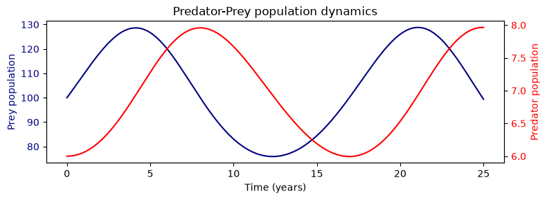

ODE solver library¶

The SciPy library comes with an ODE solver named odeint that serves as an alternative.

The basic need of odeint is for the user to implement a function that returns the array $\mathbf{y}'(t)$ . This function is thereafter passed as an argument to odeint together with the initial values of $\mathbf{y}$ and the additional arguments of the function.

def lotka_volterra(y, t, alpha, beta, delta, gamma):
    y1, y2 = y

    if delta * y1 > np.log(2):
        delta = np.log(2) / y1

    dydt = [alpha * y1 - beta * y1 * y2, delta * y1 * y2 - gamma * y2]

    return dydt

from scipy.integrate import odeint

y = odeint(lotka_volterra, y0, t, args=(alpha, beta, delta, gamma))

fig, ax1 = plt.subplots(figsize=(8, 3))
ax2 = ax1.twinx()  # instantiate a second axes that shares the same x-axis

ax1.plot(t, ppm.preys, color="navy", label="Prey")
ax2.plot(t, ppm.predators, color="red", label="Predator")

ax1.set_title("Predator-Prey population dynamics")
ax1.set_ylabel(r"Prey population", color="navy")
ax2.set_ylabel(r"Predator population", color="red")
ax1.set_xlabel(r"Time (years)")

ax1.tick_params(axis="y", labelcolor="navy")
ax2.tick_params(axis="y", labelcolor="red")

fig.tight_layout()

plt.show()

We note that the odeint and Euler solutions are in perfect agreement.

Analysis of solutions¶

While it is most natural to present the solutions to ODEs in terms of plots of state variables with respect to time, it can be revealing to plot solutions parametrically as orbitals in phase space. Let us consider the solutions to our predator–prey model with vaying initial populations.

plt.title("Phase-space plot")

plt.ylabel(r"Predators")
plt.xlabel(r"Preys")

y0_l = [[130, 7],[120, 7],[110, 7],[100, 7],]

for y0 in y0_l:

    y = odeint(lotka_volterra, y0, t, args=(alpha, beta, delta, gamma))

    plt.plot(y[:, 0], y[:, 1], "-")
    plt.plot(y[0, 0], y[0, 1], "o")

plt.show()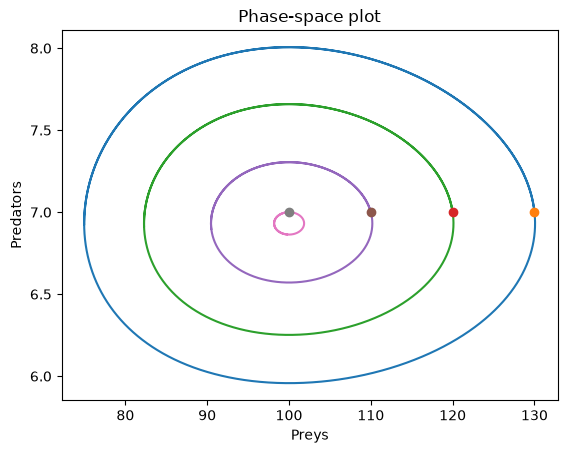

The initial populations are depicted by the solid circles in the figure and the orbitals in phase space become gradually smaller, which corresponds to reduced variations in the populations. There appears to be a central point for which populations are static (not changing in time). This point correspond mathematically to a point where the array of derivatives of the Lotka–Volterra equation is zero:

\begin{align*} \alpha y_1 - \beta y_1 y_2 & = 0 \\ \delta y_1 y_2 - \gamma y_2 & = 0 \end{align*}

(11)

This set of equations has one trivial solution in terms of zero populations but also one nontrivial solution given by

y_1 = \frac{\gamma}{\delta}; \quad y_2 = \frac{\alpha}{\beta}

(12)

With our choice of rate parameters, we get

print(f"Stable prey population    : {gamma/delta:6.1f}")
print(f"Stable predator population: {alpha/beta:6.1f}")

Stable prey population    :  100.0
Stable predator population:    6.9