PyTorch - Mathematical Modeling in Biotechnology

PyTorch is a machine learning framework based on the Torch library, used for applications such as computer vision and natural language processing. PyTorch provides two high-level features:

Tensor computing with acceleration via graphics processing units (GPUs)
Deep neural networks built on a tape-based automatic differentiation system

import torch

Tensors¶

The central data abstraction in PyTorch is given by the torch.tensor class. It represents the counterpart of the numpy.ndarray class in NumPy, and many of the respective class methods have similar syntax.

Tensor creation¶

Ways to create PyTorch tensors include:

torch.tensor()
torch.empty()
torch.zeros()
torch.ones()
torch.rand()

a = torch.rand(3, 3, dtype=torch.float32)

print(a)

tensor([[0.2752, 0.8349, 0.4992],
        [0.2107, 0.2006, 0.6319],
        [0.7102, 0.5687, 0.6047]])

By default, PyTorch tensors are populated with 32-bit (single precision) floating point numbers suitable for arithmetic operations on GPUs, but many other data types are available and include:

torch.bool
torch.int8
torch.int16
torch.int32
torch.int64
torch.half or torch.float16
torch.float
torch.double or torch.float64

A PyTorch tensor can be converted to a regular Python list.

a.tolist()

[[0.27519768476486206, 0.8349402546882629, 0.4992189407348633],
 [0.21069538593292236, 0.20064371824264526, 0.6318506598472595],
 [0.710239827632904, 0.5686625242233276, 0.6047130823135376]]

Conversely, a Python list can be converted to a PyTorch tensor.

torch.tensor(a.tolist())

tensor([[0.2752, 0.8349, 0.4992],
        [0.2107, 0.2006, 0.6319],
        [0.7102, 0.5687, 0.6047]])

Tensor operations¶

PyTorch tensors have over three hundred operations that can be performed on them, including:

torch.abs()
torch.max()
torch.mean()
torch.std()
torch.prod()
torch.unique()
torch.matmul()
torch.svd()
torch.sin()
torch.cos()
torch.flatten()

a.mean()

tensor(0.5040)

Note that a tensor with a scalar number is given in return. To instead get a Python number in return, we can perform

a.mean().item()

0.5040180683135986

NumPy bridge¶

import numpy as np

np_array = np.ones((2, 3))
pth_tensor = torch.from_numpy(np_array)

print(pth_tensor)

tensor([[1., 1., 1.],
        [1., 1., 1.]], dtype=torch.float64)

We note that the NumPy array default data type of float64 (double precision) is preserved. In fact, we merely created a pointer to the same data in memory such that a change in one object is reflected in both.

np_array[1, 2] = 2

print("Modified numpy array:\n", np_array)
print("Bridged pytorch tensor:\n", pth_tensor)

Modified numpy array:
 [[1. 1. 1.]
 [1. 1. 2.]]
Bridged pytorch tensor:
 tensor([[1., 1., 1.],
        [1., 1., 2.]], dtype=torch.float64)

A reason to create a bridge between data can e.g. be to take advantage of the easy accessible GPU acceleration available in PyTorch for scientific codes developed with NumPy.

Neural networks¶

The machine learning models in PyTorch are built as neural networks with layers of neurons. Every neuron has an associated activation level.

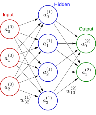
The input layer receives input data; hidden layers transform the data; and the output layer provides the results upon which model predictions are made.

The input level apart, activation levels in a given level, say $L$ , are determined from those in the previous layer by use of weights that are collected in a matrix $\boldsymbol{W}^{(L)}$ and biases that are collected in a row vector $\boldsymbol{b}^{(L)}$ .

The organization of the weights into matrix form is illustrated in figure. The neuron number in layer $L$ becomes the row index and the neuron number in layer $L-1$ becomes the column index.

A layer is referred to as linear if the weights and biases are applied in a linear transformation

\boldsymbol{a}^{(L)} = f(\boldsymbol{a}^{(L-1)} \big[\boldsymbol{W}^{(L)}\big]^T + \boldsymbol{b}^{(L)})

(1)

As indicated, to get the final activation levels also involves the elementwise operation of a (typically) nonlinear activation function, $f$ .

When instantiated, layer $L$ receives weight and bias attributes that are initialized randomly with values

-1/\sqrt{n_{L-1}} < w_{ij}^{(L)}, b_i^{(L)} < 1 / \sqrt{n_{L-1}}

(2)

where $n_{L-1}$ is the number of neurons in layer $L-1$ .

torch.manual_seed(20240305)

Input layer¶

Let us assume that we have the following input data.

a0 = torch.tensor([2.8317, 0.7713, 0.7910])

print("Input layer data:\n", a0)

Input layer data:
 tensor([2.8317, 0.7713, 0.7910])

Hidden layer¶

Layer transformation¶

The linear layer transformation is achieved with the torch.nn.Linear class.

Here we consider a transformation from an input layer with three neurons, $n_0 = 3$ , to a hidden layer with four neurons, $n_1 = 4$ .

hidden = torch.nn.Linear(3, 4, bias=True)

The weights and biases are available as attributes of the layer object.

hidden.weight

Parameter containing:
tensor([[ 0.3830,  0.3132, -0.4861],
        [ 0.3464, -0.4345, -0.4673],
        [ 0.0303,  0.3445,  0.0182],
        [-0.1550,  0.4523, -0.1824]], requires_grad=True)

hidden.bias

Parameter containing:
tensor([-0.1304, -0.0389, -0.1370, -0.2898], requires_grad=True)

We now use PyToch to perform the layer transformation of the input data.

hidden(a0)

tensor([ 0.8114, 0.2372, 0.2288, -0.5243], grad_fn=<ViewBackward0>)

We check the transformation with an explicit calculation of the linear transformation:

\boldsymbol{a}^{(0)} \big[\boldsymbol{W}^{(1)}\big]^T + \boldsymbol{b}^{(1)}

(3)

torch.matmul(a0, hidden.weight.T) + hidden.bias

tensor([ 0.8114, 0.2372, 0.2288, -0.5243], grad_fn=<AddBackward0>)

We note that the two results are identical.

Activation function¶

Now remains the application of the nonlinear activation function, $f$ , according to

\boldsymbol{a}^{(1)} =f( \boldsymbol{a}^{(0)} \big[\boldsymbol{W}^{(1)}\big]^T + \boldsymbol{b}^{(1)})

(4)

A common choice in machine learning is to adopt the rectifier linear unit function

\mathrm{ReLU}(x) = \max(0,x) = \frac{x + |x|}{2}

(5)

relu = torch.nn.ReLU()

a1 = relu(hidden(a0))

print("Hidden layer data:\n", a1)

Hidden layer data:
 tensor([0.8114, 0.2372, 0.2288, 0.0000], grad_fn=<ReluBackward0>)

The effect of the ReLU function is as anticipated, turning activation level $a^{(1)}_3$ to zero.

Output layer¶

We create the output layer as a linear layer without a nonlinear activation function.

output = torch.nn.Linear(4, 2, bias=True)

a2 = output(a1)

print("Output layer data:\n", a2)

Output layer data:
 tensor([-0.1211, -0.2292], grad_fn=<ViewBackward0>)

Network training¶

training_data = torch.tensor([-0.5, -1.0])

size = len(training_data)

Loss function¶

In the process of training the network, we need a measure of closeness between the prediction in the output layer and the correct result. This measure is given by a loss function. Several loss functions are available in PyTorch for different purposes. We will here adopt the mean square error function.

loss_mse = torch.nn.MSELoss()

loss = loss_mse(a2, training_data)

print("Loss based on mean square error:\n", loss)

Loss based on mean square error:
 tensor(0.3688, grad_fn=<MseLossBackward0>)

torch.sum((a2 - training_data) ** 2) / size

tensor(0.3688, grad_fn=<DivBackward0>)

Backpropagation¶

The gradient of the loss function with respect to weight and bias parameters are determined with a method known as backpropagation that is based on chain rule differentiation.

loss.backward()

hidden.weight.grad

tensor([[-0.7216, -0.1966, -0.2016],
        [ 0.0070,  0.0019,  0.0019],
        [ 1.2845,  0.3499,  0.3588],
        [ 0.0000,  0.0000,  0.0000]])

We note that since activation level $a_3^{(1)}$ became equal to zero in our network, the gradient with respect to weight parameters $w^{(1)}_{30}$ , $w^{(1)}_{31}$ , and $w^{(1)}_{32}$ vanish.

output.weight.grad

tensor([[0.3074, 0.0899, 0.0867, 0.0000],
        [0.6254, 0.1828, 0.1764, 0.0000]])

We note that since activation level $a_3^{(1)}$ became equal to zero in our network, the gradient with respect to weight parameters $w^{(2)}_{03}$ and $w^{(2)}_{13}$ vanish.

With access to these gradients, the parameters can be modified in a way to reduce the value of the loss function. This iterative process is referred to as training the network.

A large training data set is required in practice and an approach such as the stochastic gradient descent method can be used to update the parameter values.

Cross entropy loss function¶

In binary classification networks, the CrossEntropyLoss() function is a typical choice. The evaluation of this loss function is a bit less straightforward and since it will be subsequently used, it is here illustrated by an example.

loss_func = torch.nn.CrossEntropyLoss()

Let us assume that we have four classes in the output layer and that we are concerned with a specific item in the data set for which the correct answer is class number three.

correct_answer = torch.tensor([0.0, 0.0, 1.0, 0.0])

Let us further assume that we have made two separate predictions (one good and one bad) in the output layer leading to the following activity levels.

good_prediction = torch.tensor([0.2, 0.5, 3.1, -0.1])

bad_prediction = torch.tensor([2.0, 2.5, 1.1, -0.5])

The associated loss function values (errors) are given by:

print("good prediction loss =", loss_func(good_prediction, correct_answer))
print("bad prediction loss  =", loss_func(bad_prediction, correct_answer))

good prediction loss = tensor(0.1571)
bad prediction loss  = tensor(2.0434)

As expected, the error is deemed much larger for the bad prediction.

Let us see how PyTorch came this conclusion.

In a first step, the predictions are exponentialized, promoting large positive numbers.

good_p1 = torch.exp(good_prediction)
bad_p1 = torch.exp(bad_prediction)

print("step 1: good prediction loss =", good_p1)
print("step 1: bad prediction loss  =", bad_p1)

step 1: good prediction loss = tensor([ 1.2214,  1.6487, 22.1979,  0.9048])
step 1: bad prediction loss  = tensor([ 7.3891, 12.1825,  3.0042,  0.6065])

In a second step, a normalization is performed.

good_p2 = good_p1 / good_p1.sum()
bad_p2 = bad_p1 / bad_p1.sum()

print("step 2: good prediction loss =", good_p2)
print("step 2: bad prediction loss  =", bad_p2)

step 2: good prediction loss = tensor([0.0470, 0.0635, 0.8547, 0.0348])
step 2: bad prediction loss  = tensor([0.3187, 0.5255, 0.1296, 0.0262])

In a third step, we take the negative logarithm so that a values close to one become close to zero (low loss).

good_p3 = -torch.log(good_p2)
bad_p3 = -torch.log(bad_p2)

print("step 3: good prediction loss =", good_p3)
print("step 3: bad prediction loss  =", bad_p3)

step 3: good prediction loss = tensor([3.0571, 2.7571, 0.1571, 3.3571])
step 3: bad prediction loss  = tensor([1.1434, 0.6434, 2.0434, 3.6434])

In a forth step, we pick out the loss for the binary correct answer by means of a product.

good_p4 = good_p3 * correct_answer
bad_p4 = bad_p3 * correct_answer

print("step 4: good prediction loss =", good_p4)
print("step 4: bad prediction loss  =", bad_p4)

step 4: good prediction loss = tensor([0.0000, 0.0000, 0.1571, 0.0000])
step 4: bad prediction loss  = tensor([0.0000, 0.0000, 2.0434, 0.0000])

In a fifth step, a summation is performed to produce a scalar loss value.

print("good prediction loss =", good_p4.sum())
print("bad prediction loss  =", bad_p4.sum())

good prediction loss = tensor(0.1571)
bad prediction loss  = tensor(2.0434)

We note that the resulting losses are identical to those obtained with the PyTorch loss function.

TorchVision MNIST example¶

PyTorch offers domain-specific libraries such as TorchText, TorchVision, and TorchAudio, all of which include datasets. We will use a TorchVision dataset named MNIST.

import torchvision

Data set¶

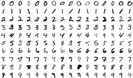
The MNIST data set consists of 28 x 28 pixel greyscale images of handwritten digits, along with labels for each image indicating which digit it represents. The data set has 60,000 images.

Loading dataset¶

mnist_dataset = torchvision.datasets.MNIST(
    root="../data_input/",
    download=True,
    train=True,
    transform=torchvision.transforms.ToTensor(),
)
print(mnist_dataset)

100%|████████████████████████████████████████████████████| 9.91M/9.91M [00:01<00:00, 7.47MB/s]
100%|█████████████████████████████████████████████████████| 28.9k/28.9k [00:00<00:00, 258kB/s]
100%|████████████████████████████████████████████████████| 1.65M/1.65M [00:00<00:00, 2.43MB/s]
100%|████████████████████████████████████████████████████| 4.54k/4.54k [00:00<00:00, 7.84MB/s]

Dataset MNIST
    Number of datapoints: 60000
    Root location: ../data_input/
    Split: Train
    StandardTransform
Transform: ToTensor()

idx_random_tensor = np.random.randint(60000)

image, label = mnist_dataset[idx_random_tensor]

print("Label:", label)
print("Dataset item:", idx_random_tensor)
print("Tensor shape:", image.shape)

Label: 5
Dataset item: 58948
Tensor shape: torch.Size([1, 28, 28])

import matplotlib.pyplot as plt

fig = plt.figure(figsize=(2,2))
plt.imshow(image[0, :, :], cmap="gray")
plt.show()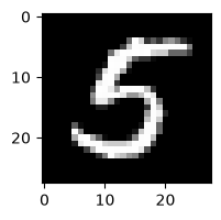

Split data set into subsets¶

In machine learning, data sets are typically divided into the three categories of training, validation, and test. We will divide data into two categories and skip the model tuning in the validation step.

training_data, test_data = torch.utils.data.random_split(mnist_dataset, [50000, 10000])

We create data loaders to be able to load the data in batches.

The shuffle option is set for the training data loader, so that the batches generated in each epoch are different. As the validation data loader is used only for evaluating the model, there is no need to shuffle these data.

batch_size = 64

train_dataloader = torch.utils.data.DataLoader(training_data, batch_size, shuffle=True)
test_dataloader = torch.utils.data.DataLoader(test_data, batch_size, shuffle=False)

Neural network model¶

Setting up the model¶

class MnistModel(torch.nn.Module):

    input_layer_dim = 28 * 28
    hidden_layer_dim = 512
    number_classes = 10

    def __init__(self):
        super().__init__()

        self.linear_stack = torch.nn.Sequential(
            torch.nn.Flatten(),
            torch.nn.Linear(self.input_layer_dim, self.hidden_layer_dim),
            torch.nn.ReLU(),
            torch.nn.Linear(self.hidden_layer_dim, self.hidden_layer_dim),
            torch.nn.ReLU(),
            torch.nn.Linear(self.hidden_layer_dim, self.number_classes),
        )

    def forward(self, x):
        y = self.linear_stack(x)
        return y

model = MnistModel()

print(model)

MnistModel(
  (linear_stack): Sequential(
    (0): Flatten(start_dim=1, end_dim=-1)
    (1): Linear(in_features=784, out_features=512, bias=True)
    (2): ReLU()
    (3): Linear(in_features=512, out_features=512, bias=True)
    (4): ReLU()
    (5): Linear(in_features=512, out_features=10, bias=True)
  )
)

Model assessment¶

A loss function is defined to quantify the model output from the reference.

loss_func = torch.nn.CrossEntropyLoss()

With this loss function, we determine the averaged loss and the percentage of correct predictions.

def test(dataloader, model):

    model.eval()

    number_correct = 0
    with torch.no_grad():
        for images, labels in dataloader:  # batches of images and labels
            output = model(images)
            number_correct += (
                (output.argmax(1) == labels).type(torch.float).sum().item()
            )

    size = len(dataloader.dataset)  # size is 10,000 in our case
    accuracy = 100 * number_correct / size  # in percent

    return accuracy

Initial model performance¶

With random parameters, we expect to prediction success of about 10%.

accuracy = test(test_dataloader, model)

print(f"Accuracy: {accuracy:>0.1f}%")

prediction_accuracies = [accuracy]  # saved in list for plotting

Accuracy: 9.8%

Model training¶

number_of_epochs = 2  # number of iterations in the training

learning_rate = 0.01  # step length in gradient descent
optimizer = torch.optim.SGD(model.parameters(), lr=learning_rate)

def train(dataloader, model, loss_func, optimizer):

    for images, labels in dataloader:  # batches of images and labels

        output = model(images)
        loss = loss_func(output, labels)

        # Back propagation
        optimizer.zero_grad()
        loss.backward()
        optimizer.step()

for epoch in range(number_of_epochs):

    print(f"Epoch ({epoch+1}/{number_of_epochs}):")

    train(train_dataloader, model, loss_func, optimizer)

    accuracy = test(test_dataloader, model)    
    prediction_accuracies.append(accuracy)

    print(f"  accuracy: {accuracy}%")

Epoch (1/2):
  accuracy: 81.56%
Epoch (2/2):
  accuracy: 87.78%

fig, ax = plt.subplots(figsize=(8, 4))

ax.plot(prediction_accuracies, "-", color="navy")
ax.plot(prediction_accuracies, "o", color="deepskyblue")

ax.set_xticks(range(0, number_of_epochs + 1))
ax.set_ylim((0, 100))
ax.set_xlim((-0.2, number_of_epochs + 0.2))
ax.grid(True)

ax.set_xlabel("Number of epochs in model training")
ax.set_ylabel("Prediction accuraciy (%)")

plt.show()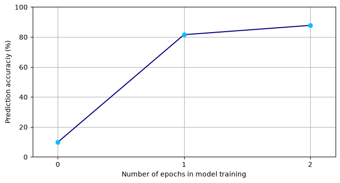

Single image prediction¶

def predict_image(x, model):

    y = model(x)

    _, prediction = torch.max(y, dim=1)

    return prediction[0].item()

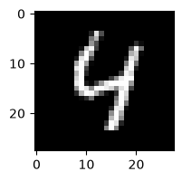
idx_random_tensor = np.random.randint(10000)

image, label = test_data[idx_random_tensor]

print("Test data set item:", idx_random_tensor)
print("Label:", label)
print("Predicted :", predict_image(image, model))

fig = plt.figure(figsize=(2,2))
plt.imshow(image[0, :, :], cmap="gray")
plt.show()

Test data set item: 2341
Label: 4
Predicted : 4

Saving and loading models¶

The model parameters (weights and biases) are returned by the state_dict() method.

The model parameters can be saved to a file.

# torch.save(model.state_dict(), "mnist-model.pth")

A saved model can be read from file.

# model = MnistModel()
# model.load_state_dict(torch.load("mnist-model.pth"))