Non-standard calculations#

In this chapter we will consider some non-standard calculations. Some can be useful but need care for practical considerations (i.e. transient X-ray spectroscopy), and some are more illustrations of alternative (but not recommended) ways of modelling spectra. Be careful before directly adopting these approaches for some practical problem.

Loading modules and routines:

import copy
import adcc
import matplotlib.pyplot as plt
import numpy as np
import veloxchem as vlx

def lorentzian(x, y, xmin, xmax, xstep, gamma):
    xi = np.arange(xmin, xmax, xstep)
    yi = np.zeros(len(xi))
    for i in range(len(xi)):
        for k in range(len(x)):
            yi[i] = yi[i] + y[k] * (gamma / 2.0) / (
                (xi[i] - x[k]) ** 2 + (gamma / 2.0) ** 2
            )
    return xi, yi

au2ev = 27.211386
* Warning * Environment variable OMP_NUM_THREADS not set.
* Warning * Setting OMP_NUM_THREADS to 4.

Transient X-ray absorption spectroscopy#

An increasingly large field of study is to use a pump-probe protocol, where some chemical reaction is initiated by some pump (typically a laser), and the dynamics are then probed using some X-ray spectroscopy. The modeling of such process is quite new, and we will here present some protocols of how such processes can be considered.

Valence-excited reference state#

By using an excited state as the references state, the X-ray absorption spectra can be considered in a manner similar to XES:

  1. Perform a ground state calculation

  2. Use the result as initial guess for a second calculation, where the occupations are changed to emulate that of the desired (valence) excited state

  3. Perform a wave function optimization with above configuration, using a constraint such as MOM to avoid a collapse to the ground state

  4. Calculate the X-ray absorption spectra of this reference state

When considering (singlet) valence-excitations of a closed-shell molecule, two different reference state spin-muliticiplicity configurations are possible:

  • Low-spin open-shell reference (LSOR), which moves an electron within the same multiplicity

  • High-spin open-shell reference (HSOR), which flips the spin of the moved electron, and thus forms a triplet reference state (when considering singlet excitations of a closed-shell system)

Note that the LSOR wave function will be heavily spin contaminated, as seen below. This has been claimed to lead to minimal errors, but care should be taken. Further note that converging to a reference state which represents the actual valence excitation is non-trivial, and may indeed be all but impossible. As such, this two-step approach is useful, but has some issues. Finally, if using correlated methods, there are some concerns that the observed relative energies are off from experimental values, which could relate to issues with using a non-Aufbau reference state.

As an example we consider the first valence-excited state of water:

Note

pyscf version - to be changed

water_xyz = """
O       0.0000000000     0.0000000000     0.1178336003
H      -0.7595754146    -0.0000000000    -0.4713344012
H       0.7595754146     0.0000000000    -0.4713344012
"""

mol = gto.Mole()
mol.atom = water_xyz
mol.basis = "6-31G"
mol.build()

print('GS:')
scf_gs = scf.UHF(mol)
scf_gs.kernel()

print('LSOR:')
mo0 = copy.deepcopy(scf_gs.mo_coeff)
occ0 = copy.deepcopy(scf_gs.mo_occ)
occ0[0][4] = 0.0
occ0[0][5] = 1.0
scf_lsor = scf.UHF(mol)
scf.addons.mom_occ(scf_lsor, mo0, occ0)
scf_lsor.kernel()

print('HSOR:')
mo0 = copy.deepcopy(scf_gs.mo_coeff)
occ0 = copy.deepcopy(scf_gs.mo_occ)
occ0[0][4] = 0.0
occ0[1][5] = 1.0
scf_hsor = scf.UHF(mol)
scf.addons.mom_occ(scf_hsor, mo0, occ0)
scf_hsor.kernel()

As can be seen, the \(\langle S^2 \rangle\) of the LSOR reference is close to 1, and thus represents an almost perfect mix of a singlet and triplet.

Calculating the valence-excitation energies and comparing it to energy differences obtained from the different reference states:

adc_gs = adcc.adc2(scf_gs, n_states=5)
adc_xas = adcc.cvs_adc2(scf_gs, n_states=5, core_orbitals=1)
adc_lsor = adcc.cvs_adc2(scf_lsor, n_states=5, core_orbitals=1)
adc_hsor = adcc.cvs_adc2(scf_hsor, n_states=5, core_orbitals=1)
print(adc_gs.describe())
print(27.2114 * (adc_gs.ground_state.energy() - adc_lsor.ground_state.energy()))
print(27.2114 * (adc_gs.ground_state.energy() - adc_hsor.ground_state.energy()))

The first allowed transition energy is relatively close to the \(\Delta\)MP2 results (as we use the MP2 energies), in particular for the LSOR. Resulting spectra can now be plotted as:

plt.figure(figsize=(6,3))
adc_xas.plot_spectrum(label="GS")
adc_lsor.plot_spectrum(label="LSOR")
adc_hsor.plot_spectrum(label="HSOR")
plt.legend()
plt.show()

We see the occurance of a lower-energy feature, representing the 1s to SOMO transition, as well as an upward shift of remaining features.

Coupling valence- and core-excited eigenstates#

  • To be added

Impact of channel restriction for TDDFT#

The influence of channel-restriction/CVS schemes for TDDFT can be considered for smaller systems by diagonalizing the full-space and CVS-space matrices, thus constructing the total global spectrum. This will not be possible for larger systems/basis sets, or for correlated method, where other CVS relaxation schemes have been used instead.

water_mol_str = """
O       0.0000000000     0.0000000000     0.1178336003
H      -0.7595754146    -0.0000000000    -0.4713344012
H       0.7595754146     0.0000000000    -0.4713344012
"""

basis = "6-31G"
vlx_mol = vlx.Molecule.read_molecule_string(water_mol_str)
vlx_bas = vlx.MolecularBasis.read(vlx_mol, basis)

scf_drv = vlx.ScfRestrictedDriver()
scf_settings = {"conv_thresh": 1.0e-6}
method_settings = {"xcfun": "b3lyp"}
scf_drv.update_settings(scf_settings, method_settings)
scf_results = scf_drv.compute(vlx_mol, vlx_bas)
Hide code cell output
* Info * Reading basis set from file: /opt/miniconda3/envs/echem/lib/python3.10/site-packages/veloxchem/basis/6-31G       
                                                                                                                          
                                              Molecular Basis (Atomic Basis)                                              
                                             ================================                                             
                                                                                                                          
                               Basis: 6-31G                                                                               
                                                                                                                          
                               Atom Contracted GTOs           Primitive GTOs                                              
                                                                                                                          
                                O   (3S,2P)                   (10S,4P)                                                    
                                H   (2S)                      (4S)                                                        
                                                                                                                          
                               Contracted Basis Functions : 13                                                            
                               Primitive Basis Functions  : 30                                                            
                                                                                                                          
                                                                                                                          
                                            Self Consistent Field Driver Setup                                            
                                           ====================================                                           
                                                                                                                          
                   Wave Function Model             : Spin-Restricted Kohn-Sham                                            
                   Initial Guess Model             : Superposition of Atomic Densities                                    
                   Convergence Accelerator         : Two Level Direct Inversion of Iterative Subspace                     
                   Max. Number of Iterations       : 50                                                                   
                   Max. Number of Error Vectors    : 10                                                                   
                   Convergence Threshold           : 1.0e-06                                                              
                   ERI Screening Scheme            : Cauchy Schwarz + Density                                             
                   ERI Screening Mode              : Dynamic                                                              
                   ERI Screening Threshold         : 1.0e-12                                                              
                   Linear Dependence Threshold     : 1.0e-06                                                              
                   Exchange-Correlation Functional : B3LYP                                                                
                   Molecular Grid Level            : 4                                                                    
                                                                                                                          
* Info * Nuclear repulsion energy: 9.1561447194 a.u.                                                                      
                                                                                                                          
* Info * Using the Libxc library (version 6.2.2).                                                                         
                                                                                                                          
         S. Lehtola, C. Steigemann, M. J.T. Oliveira, and M. A.L. Marques.,  SoftwareX 7, 1–5 (2018)
                                                                                                                          
* Info * Using the B3LYP functional.                                                                                      
                                                                                                                          
         P. J. Stephens, F. J. Devlin, C. F. Chabalowski, and M. J. Frisch.,  J. Phys. Chem. 98, 11623 (1994)
                                                                                                                          
* Info * Molecular grid with 40792 points generated in 0.03 sec.                                                          
                                                                                                                          
* Info * Overlap matrix computed in 0.00 sec.                                                                             
                                                                                                                          
* Info * Kinetic energy matrix computed in 0.00 sec.                                                                      
                                                                                                                          
* Info * Nuclear potential matrix computed in 0.00 sec.                                                                   
                                                                                                                          
* Info * Orthogonalization matrix computed in 0.00 sec.                                                                   
                                                                                                                          
* Info * SAD initial guess computed in 0.00 sec.                                                                          
                                                                                                                          
* Info * Starting Reduced Basis SCF calculation...                                                                        
* Info * ...done. SCF energy in reduced basis set: -75.983870205310 a.u. Time: 0.03 sec.                                  
                                                                                                                          
* Info * Overlap matrix computed in 0.00 sec.                                                                             
                                                                                                                          
* Info * Kinetic energy matrix computed in 0.00 sec.                                                                      
                                                                                                                          
* Info * Nuclear potential matrix computed in 0.00 sec.                                                                   
                                                                                                                          
* Info * Orthogonalization matrix computed in 0.00 sec.                                                                   
                                                                                                                          
                                                                                                                          
               Iter. |    Kohn-Sham Energy | Energy Change | Gradient Norm | Max. Gradient | Density Change               
               --------------------------------------------------------------------------------------------               
                  1       -76.384872592259    0.0000000000      0.05814060      0.01079184      0.00000000                
                  2       -76.384686594376    0.0001859979      0.07420221      0.01375784      0.03127402                
                  3       -76.385180742153   -0.0004941478      0.00038519      0.00008834      0.01650959                
                  4       -76.385180774173   -0.0000000320      0.00007657      0.00002027      0.00029092                
                  5       -76.385180774932   -0.0000000008      0.00000194      0.00000051      0.00002929                
                  6       -76.385180774934   -0.0000000000      0.00000014      0.00000003      0.00000214                
                                                                                                                          
               *** SCF converged in 6 iterations. Time: 0.36 sec.                                                         
                                                                                                                          
               Spin-Restricted Kohn-Sham:                                                                                 
               --------------------------                                                                                 
               Total Energy                       :      -76.3851807749 a.u.                                              
               Electronic Energy                  :      -85.5413254944 a.u.                                              
               Nuclear Repulsion Energy           :        9.1561447194 a.u.                                              
               ------------------------------------                                                                       
               Gradient Norm                      :        0.0000001389 a.u.                                              
                                                                                                                          
                                                                                                                          
               Ground State Information                                                                                   
               ------------------------                                                                                   
               Charge of Molecule            :  0.0                                                                       
               Multiplicity (2S+1)           :  1.0                                                                       
               Magnetic Quantum Number (M_S) :  0.0                                                                       
                                                                                                                          
                                                                                                                          
                                                 Spin Restricted Orbitals                                                 
                                                 ------------------------                                                 
                                                                                                                          
               Molecular Orbital No.   1:                                                                                 
               --------------------------                                                                                 
               Occupation: 2.000 Energy:  -19.13379 a.u.                                                                  
               (   1 O   1s  :    -1.00)                                                                                  
                                                                                                                          
               Molecular Orbital No.   2:                                                                                 
               --------------------------                                                                                 
               Occupation: 2.000 Energy:   -1.01751 a.u.                                                                  
               (   1 O   1s  :     0.21) (   1 O   2s  :    -0.46) (   1 O   3s  :    -0.45)                              
               (   1 O   1p0 :     0.15) (   2 H   1s  :    -0.15) (   3 H   1s  :    -0.15)                              
                                                                                                                          
               Molecular Orbital No.   3:                                                                                 
               --------------------------                                                                                 
               Occupation: 2.000 Energy:   -0.52917 a.u.                                                                  
               (   1 O   1p+1:     0.52) (   1 O   2p+1:     0.23) (   2 H   1s  :    -0.27)                              
               (   2 H   2s  :    -0.15) (   3 H   1s  :     0.27) (   3 H   2s  :     0.15)                              
                                                                                                                          
               Molecular Orbital No.   4:                                                                                 
               --------------------------                                                                                 
               Occupation: 2.000 Energy:   -0.35661 a.u.                                                                  
               (   1 O   2s  :     0.20) (   1 O   3s  :     0.37) (   1 O   1p0 :     0.54)                              
               (   1 O   2p0 :     0.38)                                                                                  
                                                                                                                          
               Molecular Orbital No.   5:                                                                                 
               --------------------------                                                                                 
               Occupation: 2.000 Energy:   -0.29214 a.u.                                                                  
               (   1 O   1p-1:     0.65) (   1 O   2p-1:     0.50)                                                        
                                                                                                                          
               Molecular Orbital No.   6:                                                                                 
               --------------------------                                                                                 
               Occupation: 0.000 Energy:    0.05639 a.u.                                                                  
               (   1 O   2s  :     0.15) (   1 O   3s  :     1.09) (   1 O   1p0 :    -0.29)                              
               (   1 O   2p0 :    -0.44) (   2 H   2s  :    -0.94) (   3 H   2s  :    -0.94)                              
                                                                                                                          
               Molecular Orbital No.   7:                                                                                 
               --------------------------                                                                                 
               Occupation: 0.000 Energy:    0.14625 a.u.                                                                  
               (   1 O   1p+1:    -0.42) (   1 O   2p+1:    -0.75) (   2 H   2s  :    -1.28)                              
               (   3 H   2s  :     1.28)                                                                                  
                                                                                                                          
               Molecular Orbital No.   8:                                                                                 
               --------------------------                                                                                 
               Occupation: 0.000 Energy:    0.80982 a.u.                                                                  
               (   1 O   1p+1:     0.20) (   1 O   2p+1:     0.53) (   2 H   1s  :     0.97)                              
               (   2 H   2s  :    -0.67) (   3 H   1s  :    -0.97) (   3 H   2s  :     0.67)                              
                                                                                                                          
               Molecular Orbital No.   9:                                                                                 
               --------------------------                                                                                 
               Occupation: 0.000 Energy:    0.87513 a.u.                                                                  
               (   1 O   2s  :     0.18) (   1 O   3s  :    -0.28) (   1 O   1p0 :    -0.78)                              
               (   1 O   2p0 :     0.50) (   2 H   1s  :    -0.71) (   2 H   2s  :     0.59)                              
               (   3 H   1s  :    -0.71) (   3 H   2s  :     0.59)                                                        
                                                                                                                          
               Molecular Orbital No.  10:                                                                                 
               --------------------------                                                                                 
               Occupation: 0.000 Energy:    0.88918 a.u.                                                                  
               (   1 O   1p-1:     0.96) (   1 O   2p-1:    -1.04)                                                        
                                                                                                                          

Full-space results#

For the full-space results, we construct the Hessian and property gradients:

lr_eig_solver = vlx.LinearResponseEigenSolver()
lr_eig_solver.update_settings(scf_settings, method_settings)

lr_solver = vlx.LinearResponseSolver()
lr_solver.update_settings(scf_settings, method_settings)

# Electronic Hessian
E2 = lr_eig_solver.get_e2(vlx_mol, vlx_bas, scf_results)

# Property gradients for dipole operator
V1_x, V1_y, V1_z = lr_solver.get_prop_grad("electric dipole", "xyz", vlx_mol, vlx_bas, scf_results)

# Dimension
c = int(len(E2) / 2)

# Overlap matrix
S2 = np.identity(2 * c)
S2[c : 2 * c, c : 2 * c] *= -1
* Info * Using the Libxc library (version 6.2.2).                                                                         
                                                                                                                          
         S. Lehtola, C. Steigemann, M. J.T. Oliveira, and M. A.L. Marques.,  SoftwareX 7, 1–5 (2018)
                                                                                                                          
* Info * Using the B3LYP functional.                                                                                      
                                                                                                                          
         P. J. Stephens, F. J. Devlin, C. F. Chabalowski, and M. J. Frisch.,  J. Phys. Chem. 98, 11623 (1994)
                                                                                                                          
* Info * Molecular grid with 40792 points generated in 0.03 sec.                                                          
                                                                                                                          
* Info * Processing Fock builds... (batch size: 160)                                                                      
* Info *   batch 1/1                                                                                                      

Calculating the excitation energies and oscillator strengths:

# Set up and solve eigenvalue problem
Sinv = np.linalg.inv(S2)  # for clarity - is identical
M = np.matmul(Sinv, E2)
eigs, X = np.linalg.eig(M)

# Reorder results
idx = np.argsort(eigs)
eigs = np.array(eigs)[idx]
X = np.array(X)[:, idx]

# Compute oscillator strengths
fosc = []
for i in range(int(len(eigs) / 2)):
    j = i + int(len(eigs) / 2)  # focus on excitations
    Xf = X[:, j]
    Xf = Xf / np.sqrt(np.matmul(Xf.T, np.matmul(S2, Xf)))
    tm = np.dot(Xf, V1_x) ** 2 + np.dot(Xf, V1_y) ** 2 + np.dot(Xf, V1_z) ** 2
    fosc.append(tm * 2.0 / 3.0 * eigs[j])

CVS-space results#

The CVS-space results can be obtained as discussed in this section, or directly using the VeloxChem implementation:

lr_eig_solver.core_excitation = True
lr_eig_solver.num_core_orbitals = 1
lr_eig_solver.nstates = 3
vlx_cvs_results = lr_eig_solver.compute(vlx_mol, vlx_bas, scf_results)
Hide code cell output
                                                                                                                          
                                                                                                                          
                                            Linear Response EigenSolver Setup                                             
                                           ===================================                                            
                                                                                                                          
                               Number of States                : 3                                                        
                               Max. Number of Iterations       : 150                                                      
                               Convergence Threshold           : 1.0e-06                                                  
                               ERI Screening Scheme            : Cauchy Schwarz + Density                                 
                               ERI Screening Threshold         : 1.0e-12                                                  
                               Exchange-Correlation Functional : B3LYP                                                    
                               Molecular Grid Level            : 4                                                        
                                                                                                                          
* Info * Using the Libxc library (version 6.2.2).                                                                         
                                                                                                                          
         S. Lehtola, C. Steigemann, M. J.T. Oliveira, and M. A.L. Marques.,  SoftwareX 7, 1–5 (2018)
                                                                                                                          
* Info * Using the B3LYP functional.                                                                                      
                                                                                                                          
         P. J. Stephens, F. J. Devlin, C. F. Chabalowski, and M. J. Frisch.,  J. Phys. Chem. 98, 11623 (1994)
                                                                                                                          
* Info * Molecular grid with 40792 points generated in 0.02 sec.                                                          
                                                                                                                          
* Info * Processing Fock builds... (batch size: 6)                                                                        
* Info *   batch 1/1                                                                                                      
                                                                                                                          
* Info * 3 gerade trial vectors in reduced space                                                                          
* Info * 3 ungerade trial vectors in reduced space                                                                        
                                                                                                                          
* Info * 1.64 kB of memory used for subspace procedure on the master node                                                 
* Info * 2.34 GB of memory available for the solver on the master node                                                    
                                                                                                                          
               *** Iteration:   1 * Residuals (Max,Min): 9.82e-02 and 2.73e-02                                            
                                                                                                                          
               Excitation 1   :     19.11351025 Residual Norm: 0.09818089                                                 
               Excitation 2   :     19.18647630 Residual Norm: 0.09204895                                                 
               Excitation 3   :     19.84616908 Residual Norm: 0.02730824                                                 
                                                                                                                          
* Info * Processing Fock builds... (batch size: 4)                                                                        
* Info *   batch 1/1                                                                                                      
                                                                                                                          
* Info * 5 gerade trial vectors in reduced space                                                                          
* Info * 5 ungerade trial vectors in reduced space                                                                        
                                                                                                                          
* Info * 2.32 kB of memory used for subspace procedure on the master node                                                 
* Info * 2.34 GB of memory available for the solver on the master node                                                    
                                                                                                                          
               *** Iteration:   2 * Residuals (Max,Min): 1.01e-02 and 1.93e-14                                            
                                                                                                                          
               Excitation 1   :     19.11231928 Residual Norm: 0.01012702                                                 
               Excitation 2   :     19.18487023 Residual Norm: 0.00000000   converged                                     
               Excitation 3   :     19.84589976 Residual Norm: 0.00000000   converged                                     
                                                                                                                          
* Info * Processing Fock builds... (batch size: 2)                                                                        
* Info *   batch 1/1                                                                                                      
                                                                                                                          
* Info * 6 gerade trial vectors in reduced space                                                                          
* Info * 6 ungerade trial vectors in reduced space                                                                        
                                                                                                                          
* Info * 2.58 kB of memory used for subspace procedure on the master node                                                 
* Info * 2.34 GB of memory available for the solver on the master node                                                    
                                                                                                                          
               *** Iteration:   3 * Residuals (Max,Min): 2.51e-04 and 2.09e-14                                            
                                                                                                                          
               Excitation 1   :     19.11231840 Residual Norm: 0.00025135                                                 
               Excitation 2   :     19.18487023 Residual Norm: 0.00000000   converged                                     
               Excitation 3   :     19.84589976 Residual Norm: 0.00000000   converged                                     
                                                                                                                          
* Info * Processing Fock builds... (batch size: 2)                                                                        
* Info *   batch 1/1                                                                                                      
                                                                                                                          
* Info * 7 gerade trial vectors in reduced space                                                                          
* Info * 7 ungerade trial vectors in reduced space                                                                        
                                                                                                                          
* Info * 2.66 kB of memory used for subspace procedure on the master node                                                 
* Info * 2.34 GB of memory available for the solver on the master node                                                    
                                                                                                                          
               *** Iteration:   4 * Residuals (Max,Min): 5.84e-14 and 1.15e-14                                            
                                                                                                                          
               Excitation 1   :     19.11231840 Residual Norm: 0.00000000   converged                                     
               Excitation 2   :     19.18487023 Residual Norm: 0.00000000   converged                                     
               Excitation 3   :     19.84589976 Residual Norm: 0.00000000   converged                                     
                                                                                                                          
               *** Linear response converged in 4 iterations. Time: 0.54 sec                                              
                                                                                                                          
                                                                                                                          
               Electric Transition Dipole Moments (dipole length, a.u.)                                                   
               --------------------------------------------------------                                                   
                                                X            Y            Z                                               
               Excited State    S1:     -0.000000    -0.000000     0.036994                                               
               Excited State    S2:     -0.053332     0.000000    -0.000000                                               
               Excited State    S3:     -0.026326    -0.000000    -0.000000                                               
                                                                                                                          
               Electric Transition Dipole Moments (dipole velocity, a.u.)                                                 
               ----------------------------------------------------------                                                 
                                                X            Y            Z                                               
               Excited State    S1:     -0.000000    -0.000000     0.037908                                               
               Excited State    S2:     -0.054574     0.000000    -0.000000                                               
               Excited State    S3:     -0.023365    -0.000000    -0.000000                                               
                                                                                                                          
               Magnetic Transition Dipole Moments (a.u.)                                                                  
               -----------------------------------------                                                                  
                                                X            Y            Z                                               
               Excited State    S1:      0.000000    -0.000000    -0.000000                                               
               Excited State    S2:     -0.000000    -0.116020    -0.000000                                               
               Excited State    S3:      0.000000    -0.051026    -0.000000                                               
                                                                                                                          
               One-Photon Absorption                                                                                      
               ---------------------                                                                                      
               Excited State    S1:     19.11231840 a.u.    520.07268 eV    Osc.Str.    0.0174                            
               Excited State    S2:     19.18487023 a.u.    522.04691 eV    Osc.Str.    0.0364                            
               Excited State    S3:     19.84589976 a.u.    540.03444 eV    Osc.Str.    0.0092                            
                                                                                                                          
               Electronic Circular Dichroism                                                                              
               -----------------------------                                                                              
               Excited State    S1:     Rot.Str.      0.000000 a.u.     0.0000 [10**(-40) cgs]                            
               Excited State    S2:     Rot.Str.      0.000000 a.u.     0.0000 [10**(-40) cgs]                            
               Excited State    S3:     Rot.Str.     -0.000000 a.u.    -0.0000 [10**(-40) cgs]                            
                                                                                                                          
               Character of excitations:                                                                                  
                                                                                                                          
               Excited state 1                                                                                            
               ---------------                                                                                            
               core_1   -> LUMO        -0.9993                                                                            
                                                                                                                          
               Excited state 2                                                                                            
               ---------------                                                                                            
               core_1   -> LUMO+1       0.9984                                                                            
                                                                                                                          
               Excited state 3                                                                                            
               ---------------                                                                                            
               core_1   -> LUMO+2      -0.9986                                                                            
                                                                                                                          

Comparison#

Comparing the obtained spectra:

plt.figure(figsize=(6,3))

x, y = eigs[int(len(eigs) / 2) :], fosc
x1, y1 = lorentzian(x, y, 518 / au2ev, 525 / au2ev, 0.001, 0.3 / au2ev)
plt.plot(x1 * au2ev, y1)

x, y = vlx_cvs_results['eigenvalues'], vlx_cvs_results['oscillator_strengths']
x2, y2 = lorentzian(x, y, 518 / au2ev, 525 / au2ev, 0.001, 0.3 / au2ev)
plt.plot(x2 * au2ev, y2, linestyle='--')

plt.plot(x1 * au2ev, 10*(y1 - y2), linestyle=':')

plt.legend(("Full-space", "CVS-space", "Difference x10"))
plt.tight_layout()
plt.show()
../../_images/5465b92b00b7855c16ea4bfd64ce12b53464ca917e0abcbbf91a2a69966b0ead.png

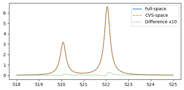
We note a small difference between the two approaches. This difference has some dependence on the basis set, but will continue to be small for the K-edge.

Ionization energies from XAS#

Can model the ionization energy by targetting excitations to extremely diffuse molecular orbital. Here: consider both spectrum and IE of water, at a CVS-ADC(2)-x/6-31G[+diffuse] level of theory.

  • To be added

Ionization energies from XES#

Can model the ionization energy by targetting decays from an extremely diffuse molecular orbital, with a core-electron already moved to it. The need of preparing this state makes the approach rather useless, but it can still provide insight into relaxation effects of XES. Here: consider the IE of water, at a CVS-ADC(2)/6-31G[+diffuse] level of theory.

  • To be added

XES considered in reverse#

Instead of modeling XES by looking at the (negative) eigenstates of a core-hole reference state, it is possible to use a valence-hole reference state, and then consider core-excitations into this hole. This thus models the XES process more from the point of view of XAS, i.e. in reverse. However, this approach presupposes:

  1. That a single-particle picture works quite well, and that specific valence-hole will yield reasonable representations of the valence-hole left following decay into a core-hole

  2. That the valence-hole can be converged well, and that the different (non-orthogonal) reference states from each calculation are sufficiently consistent with each other

Furthermore, the calculation is made more tedious, as

  1. It requires one explicit calculation per state

As such, this approach is by not suggested for practical calculations, but it does illustrate the ease of which such exotic calculations can be run, as well as teach us something about the relaxation of core-transitions.

Considering the X-ray emission spectra of water, we create valence-holes in the four frontier valence MOs and construct a spectrum from this:

Note

pyscf version - to be changed

# Containers for resulting energies and intensities
xes_rev_E = []
xes_rev_f = []

# Perform unrestricted SCF calculation
scf_res = scf.UHF(mol)
scf_res.kernel()

# Copy molecular orbital coefficients
mo0 = copy.deepcopy(scf_res.mo_coeff)

# Reference calculation from core-hole
occ0 = copy.deepcopy(scf_res.mo_occ)
occ0[0][0] = 0.0
scf_ion = scf.UHF(mol)
scf.addons.mom_occ(scf_ion, mo0, occ0)
scf_ion.kernel()
adc_xes = adcc.adc2(scf_ion, n_states=4)
xes_E = -au2ev * adc_xes.excitation_energy
xes_f = adc_xes.oscillator_strength

for i in range(4):
    occ0 = copy.deepcopy(scf_res.mo_occ)
    occ0[0][4 - i] = 0.0
    # Perform unrestricted SCF calculation with MOM constraint
    scf_ion = scf.UHF(mol)
    scf.addons.mom_occ(scf_ion, mo0, occ0)
    scf_ion.kernel()
    # Perform ADC calculation of first four states
    adc_xes = adcc.cvs_adc2(scf_ion, n_states=1, core_orbitals=1)
    xes_rev_E.append(au2ev * adc_xes.excitation_energy)
    xes_rev_f.append(adc_xes.oscillator_strength)

Comparing the two different spectra:

plt.figure(figsize=(6, 3))
xi, yi = lorentzian(xes_E, xes_f, 518, 534, 0.01, 0.5)
plt.plot(xi, yi)
xi, yi = lorentzian(xes_rev_E, xes_rev_f, 518, 534, 0.01, 0.5)
plt.plot(xi, yi)
plt.legend(("From core-hole", "From valence-hole"))
plt.tight_layout()
plt.show()
../../_images/xes_reverse.svg