Reparameterize force fields#
The MMForceFieldGenerator class in VeloxChem provides a number of functions to manipulate topology files. As an example, we consider the optimization of the force field parameters for a dihedral angle of a thiophene-based optical ligand named HS-276.
Load the required modules and the equilibrium geometry:
import veloxchem as vlx
import numpy as np

# load B3LYP optimized geometry in the xyz format
molecule = vlx.Molecule.read_xyz_file("../../data/md/hs276.xyz")
molecule.show(atom_indices=True, width=600, height=450)
3Dmol.js failed to load for some reason. Please check your browser console for error messages.
We here consider the dihedral angle between the two thiophene rings, which corresponds to the rotation around bond 21-22.
The dihedral potential curves will be plotted using force field parameters from the general amber forcefield (GAFF) database, as compared to QM results. The force field will then be changed to better fit this potential.
Create the initial force field#
Initialize an MMForceFieldGenerator object and generate initial force field with pre-calculated RESP charges:
resp_chg = np.array([
    0.014967, 0.224409, 0.089489, -0.551618, 0.153050, 0.106847, -0.315042,
    0.165854, 0.206441, -0.425163, 0.225816, -0.039099, 0.179377, 0.002119,
    0.014483, -0.043666, -0.230202, 0.165960, -0.071404, 0.188598, -0.044661,
    0.088786, -0.173586, 0.175730, -0.089376, 0.164515, -0.118573, -0.150541,
    0.736497, -0.570770, -0.273724, -0.144051, 0.112846, 0.112846, 0.112846
])

ff_gen = vlx.MMForceFieldGenerator()
ff_gen.partial_charges = resp_chg
ff_gen.create_topology(molecule)
* Info * Using GAFF (v2.11) parameters.
         Reference: J. Wang, R. M. Wolf, J. W. Caldwell, P. A. Kollman, D. A. Case, J. Comput. Chem. 2004,
         25, 1157-1174.
* Info * Updated bond angle 1-9-10 (ca-ca-cc) to 107.217 deg
* Info * Updated bond angle 1-14-15 (ca-na-cc) to 126.641 deg
* Info * Updated bond angle 2-1-14 (ca-ca-na) to 131.687 deg
* Info * Updated bond angle 7-9-10 (ca-ca-cc) to 135.297 deg
* Info * Updated bond angle 9-1-14 (ca-ca-na) to 107.608 deg
* Info * Updated bond angle 14-15-17 (na-cc-cd) to 128.324 deg
* Info * Updated bond angle 19-21-22 (cd-cc-cc) to 129.220 deg
* Info * Updated bond angle 21-22-23 (cc-cc-cd) to 128.571 deg
Reparameterize the force field#
Use the reparameterize_dihedrals method to fit dihedral parameters to QM scan. If you would like to see more output during the fitting, set verbose to True.
ff_gen.reparameterize_dihedrals(rotatable_bond=(21,22),
                                scan_file="../../data/md/27-22-21-16.xyz",
                                visualize=True,
                                verbose=False)
                                          VeloxChem Dihedral Reparameterization
                                         =======================================

* Info * Rotatable bond selected: 21-22
* Info * Dihedrals involved:[[16, 21, 22, 23], [16, 21, 22, 27], [19, 21, 22, 23], [19, 21, 22, 27]]

* Info * Reading QM scan from file...
* Info *   ../../data/md/27-22-21-16.xyz

* Info * Performing dihedral scan for MM baseline by excluding the involved dihedral barriers...
* Info * Target dihedral angle: 16-21-22-27
* Info * Dihedral barriers [4.184 4.184 4.184 4.184] will be used as initial guess.
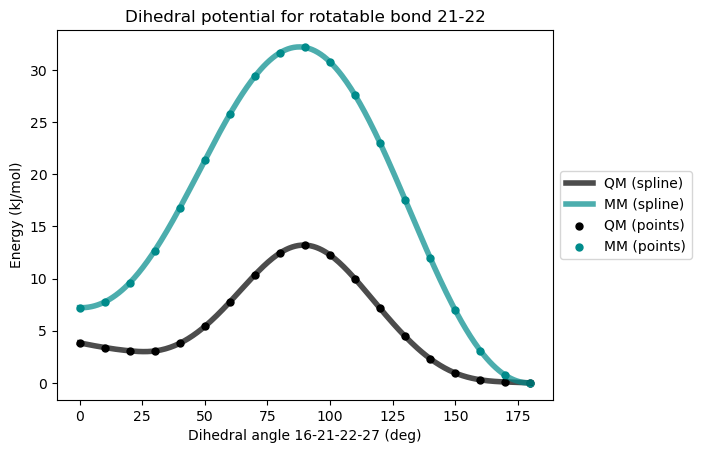
* Info * Validating the initial force field...
* Info * Dihedral MM energy(rel) QM energy(rel) diff
* Info * ---------------------------------------------------------------
* Info * 0.0 deg 7.214 kJ/mol 3.836 kJ/mol 3.378
* Info * 10.0 deg 7.759 kJ/mol 3.392 kJ/mol 4.367
* Info * 20.0 deg 9.591 kJ/mol 3.074 kJ/mol 6.517
* Info * 30.0 deg 12.689 kJ/mol 3.059 kJ/mol 9.630
* Info * 40.0 deg 16.775 kJ/mol 3.796 kJ/mol 12.978
* Info * 50.0 deg 21.348 kJ/mol 5.416 kJ/mol 15.931
* Info * 60.0 deg 25.777 kJ/mol 7.761 kJ/mol 18.016
* Info * 70.0 deg 29.406 kJ/mol 10.365 kJ/mol 19.041
* Info * 80.0 deg 31.668 kJ/mol 12.461 kJ/mol 19.208
* Info * 90.0 deg 32.174 kJ/mol 13.214 kJ/mol 18.959
* Info * 100.0 deg 30.774 kJ/mol 12.264 kJ/mol 18.511
* Info * 110.0 deg 27.589 kJ/mol 9.969 kJ/mol 17.620
* Info * 120.0 deg 22.989 kJ/mol 7.136 kJ/mol 15.853
* Info * 130.0 deg 17.549 kJ/mol 4.450 kJ/mol 13.099
* Info * 140.0 deg 11.970 kJ/mol 2.316 kJ/mol 9.654
* Info * 150.0 deg 6.956 kJ/mol 0.943 kJ/mol 6.014
* Info * 160.0 deg 3.089 kJ/mol 0.294 kJ/mol 2.795
* Info * 170.0 deg 0.727 kJ/mol 0.087 kJ/mol 0.640
* Info * 180.0 deg 0.000 kJ/mol 0.000 kJ/mol 0.000
* Info * Summary of validation
* Info * ---------------------
* Info * Maximum difference: 19.208 kJ/mol
* Info * Standard deviation: 6.676 kJ/mol
* Info * Fitting the dihedral parameters...
* Info * Optimizing dihedral via least squares fitting...
* Info * New fitted barriers: [1.85974046 1.85974046 1.85974046 1.85974046]
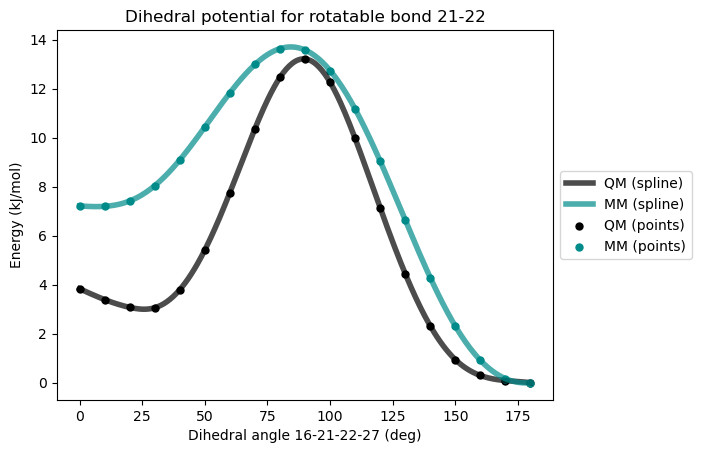
* Info * Validating the fitted force field...
* Info * Dihedral MM energy(rel) QM energy(rel) diff
* Info * ---------------------------------------------------------------
* Info * 0.0 deg 7.214 kJ/mol 3.836 kJ/mol 3.378
* Info * 10.0 deg 7.198 kJ/mol 3.392 kJ/mol 3.806
* Info * 20.0 deg 7.416 kJ/mol 3.074 kJ/mol 4.342
* Info * 30.0 deg 8.040 kJ/mol 3.059 kJ/mol 4.982
* Info * 40.0 deg 9.092 kJ/mol 3.796 kJ/mol 5.295
* Info * 50.0 deg 10.436 kJ/mol 5.416 kJ/mol 5.020
* Info * 60.0 deg 11.831 kJ/mol 7.761 kJ/mol 4.070
* Info * 70.0 deg 12.987 kJ/mol 10.365 kJ/mol 2.622
* Info * 80.0 deg 13.635 kJ/mol 12.461 kJ/mol 1.174
* Info * 90.0 deg 13.579 kJ/mol 13.214 kJ/mol 0.365
* Info * 100.0 deg 12.741 kJ/mol 12.264 kJ/mol 0.477
* Info * 110.0 deg 11.170 kJ/mol 9.969 kJ/mol 1.201
* Info * 120.0 deg 9.043 kJ/mol 7.136 kJ/mol 1.907
* Info * 130.0 deg 6.638 kJ/mol 4.450 kJ/mol 2.187
* Info * 140.0 deg 4.287 kJ/mol 2.316 kJ/mol 1.971
* Info * 150.0 deg 2.308 kJ/mol 0.943 kJ/mol 1.365
* Info * 160.0 deg 0.914 kJ/mol 0.294 kJ/mol 0.620
* Info * 170.0 deg 0.166 kJ/mol 0.087 kJ/mol 0.079
* Info * 180.0 deg 0.000 kJ/mol 0.000 kJ/mol 0.000
* Info * Summary of validation
* Info * ---------------------
* Info * Maximum difference: 5.295 kJ/mol
* Info * Standard deviation: 1.748 kJ/mol
* Info * Dihedral MM parameters have been reparameterized and updated in the topology.
{'dihedral_angles': array([  0.,  10.,  20.,  30.,  40.,  50.,  60.,  70.,  80.,  90., 100.,
        110., 120., 130., 140., 150., 160., 170., 180.]),
 'qm_scan_kJpermol': array([ 3.83585497,  3.39214553,  3.07446008,  3.05870708,  3.79647248,
         5.41640576,  7.76097693, 10.36547258, 12.46062129, 13.21413969,
        12.26370882,  9.96902213,  7.13610802,  4.45022189,  2.31569068,
         0.94255437,  0.29405596,  0.08664149,  0.        ]),
 'mm_scan_kJpermol': array([ 7.21418919,  7.19801593,  7.41635263,  8.04032619,  9.09192951,
        10.4364501 , 11.83101811, 12.98719441, 13.63501056, 13.57943482,
        12.74094985, 11.16995926,  9.04311985,  6.63759815,  4.28718943,
         2.30765762,  0.91439219,  0.16610112,  0.        ]),
 'maximum_difference': 5.295457028657646,
 'standard_deviation': 1.7480689650635666}
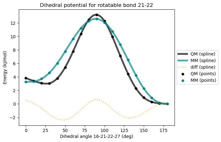
It is not uncommon that the existing dihedral terms in the force field are not sufficient to reproduce the QM potential. Here we can try adding more dihedral terms to the force field, and then redo the fitting. In this particular case we would like to lower the MM energy at 0\(^{\circ}\) so that it matches the QM energy better. This corresponds to adding a dihedral term with periodicity 1 and phase 180\(^{\circ}\). The barrier can be set to 0 since it will be fitted.
ff_gen.add_dihedral((16, 21, 22, 27), barrier=0.0, phase=180.0, periodicity=1)
* Info * Added dihedral 16-21-22-27
After adding the dihedral term we can redo the fitting. This time we can skip the initial validation step by setting initial_validation to False, since we already know how the MM potential energy curve looks. We can also set show_diff to True so that the difference between QM and MM energies will be plotted after the fitting.
ff_gen.reparameterize_dihedrals(rotatable_bond=(21,22),
                                scan_file="../../data/md/27-22-21-16.xyz",
                                visualize=True,
                                verbose=False,
                                initial_validation=False,
                                show_diff=True)
                                          VeloxChem Dihedral Reparameterization
                                         =======================================

* Info * Rotatable bond selected: 21-22
* Info * Dihedrals involved:[[16, 21, 22, 23], [16, 21, 22, 27], [19, 21, 22, 23], [19, 21, 22, 27]]

* Info * Reading QM scan from file...
* Info *   ../../data/md/27-22-21-16.xyz

* Info * Performing dihedral scan for MM baseline by excluding the involved dihedral barriers...
* Info * Target dihedral angle: 16-21-22-27

* Info * Dihedral barriers [1.85974046 1.85974046 0.         1.85974046 1.85974046] will be used as initial guess.

* Info * Fitting the dihedral parameters...
* Info * Optimizing dihedral via least squares fitting...
* Info * New fitted barriers: [1.98224593 1.98224593 1.96583572 1.98224593 1.98224593]

* Info * Validating the fitted force field...

* Info *       Dihedral      MM energy(rel)      QM energy(rel)       diff
* Info *   ---------------------------------------------------------------
* Info *        0.0 deg        3.283 kJ/mol        3.836 kJ/mol     -0.553
* Info *       10.0 deg        3.326 kJ/mol        3.392 kJ/mol     -0.066
* Info *       20.0 deg        3.718 kJ/mol        3.074 kJ/mol      0.643
* Info *       30.0 deg        4.617 kJ/mol        3.059 kJ/mol      1.558
* Info *       40.0 deg        6.025 kJ/mol        3.796 kJ/mol      2.229
* Info *       50.0 deg        7.782 kJ/mol        5.416 kJ/mol      2.366
* Info *       60.0 deg        9.617 kJ/mol        7.761 kJ/mol      1.856
* Info *       70.0 deg       11.214 kJ/mol       10.365 kJ/mol      0.849
* Info *       80.0 deg       12.278 kJ/mol       12.461 kJ/mol     -0.182
* Info *       90.0 deg       12.594 kJ/mol       13.214 kJ/mol     -0.620
* Info *      100.0 deg       12.067 kJ/mol       12.264 kJ/mol     -0.197
* Info *      110.0 deg       10.742 kJ/mol        9.969 kJ/mol      0.773
* Info *      120.0 deg        8.795 kJ/mol        7.136 kJ/mol      1.659
* Info *      130.0 deg        6.510 kJ/mol        4.450 kJ/mol      2.060
* Info *      140.0 deg        4.232 kJ/mol        2.316 kJ/mol      1.917
* Info *      150.0 deg        2.289 kJ/mol        0.943 kJ/mol      1.347
* Info *      160.0 deg        0.910 kJ/mol        0.294 kJ/mol      0.616
* Info *      170.0 deg        0.166 kJ/mol        0.087 kJ/mol      0.079
* Info *      180.0 deg        0.000 kJ/mol        0.000 kJ/mol      0.000

* Info * Summary of validation
* Info * ---------------------
* Info * Maximum difference: 2.366 kJ/mol
* Info * Standard deviation: 0.967 kJ/mol
* Info * Dihedral MM parameters have been reparameterized and updated in the topology.
{'dihedral_angles': array([  0.,  10.,  20.,  30.,  40.,  50.,  60.,  70.,  80.,  90., 100.,
        110., 120., 130., 140., 150., 160., 170., 180.]),
 'qm_scan_kJpermol': array([ 3.83585497,  3.39214553,  3.07446008,  3.05870708,  3.79647248,
         5.41640576,  7.76097693, 10.36547258, 12.46062129, 13.21413969,
        12.26370882,  9.96902213,  7.13610802,  4.45022189,  2.31569068,
         0.94255437,  0.29405596,  0.08664149,  0.        ]),
 'mm_scan_kJpermol': array([ 3.28251776,  3.32576189,  3.71787894,  4.61703774,  6.02510674,
         7.78211284,  9.61729737, 11.21440371, 12.27830288, 12.59364287,
        12.06696976, 10.74187939,  8.79523482,  6.51049056,  4.23220172,
         2.28929651,  0.91048114,  0.1657876 ,  0.        ]),
 'maximum_difference': 2.3657070819803483,
 'standard_deviation': 0.967008494063023}
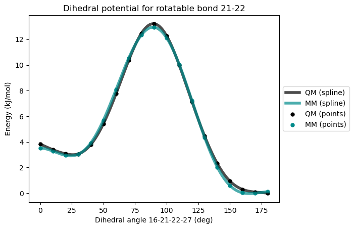
Now we get better agreement between QM and MM energies. Since the difference between QM and MM is also plotted, we can tell that the MM energies can be brought closer to QM energies by adding one more dihedral term with periodicity 4 and phase 0\(^{\circ}\).
ff_gen.add_dihedral((16, 21, 22, 27), barrier=0.0, phase=0.0, periodicity=4)
* Info * Added dihedral 16-21-22-27
ff_gen.reparameterize_dihedrals(rotatable_bond=(21,22),
                                scan_file="../../data/md/27-22-21-16.xyz",
                                visualize=True,
                                verbose=False,
                                initial_validation=False)
                                          VeloxChem Dihedral Reparameterization
                                         =======================================

* Info * Rotatable bond selected: 21-22
* Info * Dihedrals involved:[[16, 21, 22, 23], [16, 21, 22, 27], [19, 21, 22, 23], [19, 21, 22, 27]]

* Info * Reading QM scan from file...
* Info *   ../../data/md/27-22-21-16.xyz

* Info * Performing dihedral scan for MM baseline by excluding the involved dihedral barriers...
* Info * Target dihedral angle: 16-21-22-27

* Info * Dihedral barriers [1.98224593 1.98224593 1.96583572 0.         1.98224593 1.98224593] will be used as initial guess.

* Info * Fitting the dihedral parameters...
* Info * Optimizing dihedral via least squares fitting...
* Info * New fitted barriers: [2.00275023 2.00275023 1.9033555  1.23767888 2.00275023 2.00275023]

* Info * Validating the fitted force field...

* Info *       Dihedral      MM energy(rel)      QM energy(rel)       diff
* Info *   ---------------------------------------------------------------
* Info *        0.0 deg        3.525 kJ/mol        3.836 kJ/mol     -0.310
* Info *       10.0 deg        3.283 kJ/mol        3.392 kJ/mol     -0.109
* Info *       20.0 deg        2.953 kJ/mol        3.074 kJ/mol     -0.121
* Info *       30.0 deg        3.036 kJ/mol        3.059 kJ/mol     -0.023
* Info *       40.0 deg        3.920 kJ/mol        3.796 kJ/mol      0.124
* Info *       50.0 deg        5.698 kJ/mol        5.416 kJ/mol      0.282
* Info *       60.0 deg        8.095 kJ/mol        7.761 kJ/mol      0.334
* Info *       70.0 deg       10.538 kJ/mol       10.365 kJ/mol      0.173
* Info *       80.0 deg       12.339 kJ/mol       12.461 kJ/mol     -0.122
* Info *       90.0 deg       12.938 kJ/mol       13.214 kJ/mol     -0.276
* Info *      100.0 deg       12.106 kJ/mol       12.264 kJ/mol     -0.158
* Info *      110.0 deg       10.023 kJ/mol        9.969 kJ/mol      0.054
* Info *      120.0 deg        7.211 kJ/mol        7.136 kJ/mol      0.075
* Info *      130.0 deg        4.346 kJ/mol        4.450 kJ/mol     -0.104
* Info *      140.0 deg        2.032 kJ/mol        2.316 kJ/mol     -0.284
* Info *      150.0 deg        0.600 kJ/mol        0.943 kJ/mol     -0.343
* Info *      160.0 deg        0.029 kJ/mol        0.294 kJ/mol     -0.265
* Info *      170.0 deg        0.000 kJ/mol        0.087 kJ/mol     -0.087
* Info *      180.0 deg        0.118 kJ/mol        0.000 kJ/mol      0.118

* Info * Summary of validation
* Info * ---------------------
* Info * Maximum difference: 0.343 kJ/mol
* Info * Standard deviation: 0.196 kJ/mol
* Info * Dihedral MM parameters have been reparameterized and updated in the topology.
{'dihedral_angles': array([  0.,  10.,  20.,  30.,  40.,  50.,  60.,  70.,  80.,  90., 100.,
        110., 120., 130., 140., 150., 160., 170., 180.]),
 'qm_scan_kJpermol': array([ 3.83585497,  3.39214553,  3.07446008,  3.05870708,  3.79647248,
         5.41640576,  7.76097693, 10.36547258, 12.46062129, 13.21413969,
        12.26370882,  9.96902213,  7.13610802,  4.45022189,  2.31569068,
         0.94255437,  0.29405596,  0.08664149,  0.        ]),
 'mm_scan_kJpermol': array([ 3.525357  ,  3.2830363 ,  2.95338033,  3.03599648,  3.92038683,
         5.69817608,  8.09540393, 10.53821999, 12.33903773, 12.93803623,
        12.10600545, 10.02295668,  7.21086116,  4.34623078,  2.03175656,
         0.60003634,  0.02855813,  0.        ,  0.1178788 ]),
 'maximum_difference': 0.34251803167438954,
 'standard_deviation': 0.19571843656210797}
Save the force field to file#
Use write_gromacs_files or write_openmm_files to write the force field to files.
ff_gen.write_gromacs_files('hs276')