Optimization and normal modes#
In this section we will see how to visualize geometry optimization trajectories, as well as molecular vibration modes using py3Dmol.
Geometry optimization#
import veloxchem as vlx
import py3Dmol as p3d
from matplotlib import pyplot as plt
import numpy as np
import ipywidgets
import h5py
Let’s assume we have run the geometry optimization and saved all the steps in xyz format in a file. To animate the optimization trajectory we first need a routine which reads the configurations from file.
def read_xyz_file(file_name):
    """Reads all the configurations from an xyz geometry optimization file."""
    xyz_file = open(file_name, "r")
    data = xyz_file.read()
    xyz_file.close()

    xyz_file = open(file_name, "r")
    i = 0
    steps = []
    energies = []
    for line in xyz_file:
        if "Energy" in line:
            steps.append(i)
            i += 1
            parts = line.split()
            energy = float(parts[-1])
            energies.append(energy)
    xyz_file.close()

    return data, steps, energies
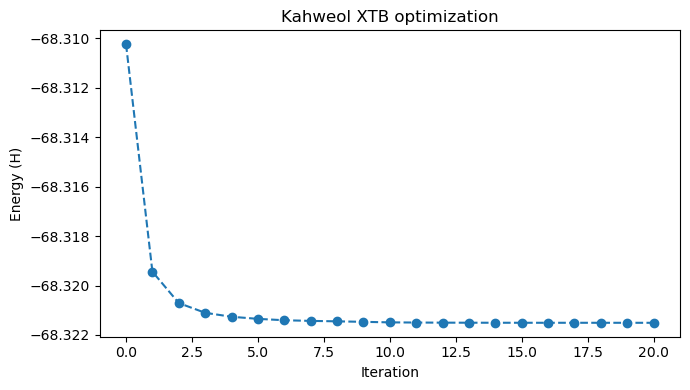
Using this routine, we can plot the energies during optimization, as well as animate the trajectory.
xyz_file_name = '../../data/md/kahweol_optim.xyz'
xyz_data, steps, energies = read_xyz_file(xyz_file_name)

# Plot the energies
plt.figure(figsize=(7,4))
plt.plot(steps, energies,'o--')
plt.xlabel('Iteration')
plt.ylabel('Energy (H)')
plt.title("Kahweol XTB optimization")
plt.tight_layout(); plt.show()

# and animate the optimization
viewer = p3d.view(width=600, height=300)
viewer.addModelsAsFrames(xyz_data)
viewer.animate({"loop": "forward"})

viewer.setViewStyle({"style": "outline", "width": 0.05})
viewer.setStyle({"stick": {}, "sphere": {"scale": 0.25}})

viewer.show()
3Dmol.js failed to load for some reason. Please check your browser console for error messages.
If instead we would like to see each configuration individually, we can create an interactive widget with a slider. As in the previous section, we need a routine which reads an individual configuration at a time and returns the corresponding py3Dmol viewer.
def read_xyz_index(file_name, index=0):
    """Reads one configuration defined by its index from the xyz optimization file."""
    xyz_file = open(file_name, "r")
    current_index = 0
    data = ""

    # Read the number of atoms from the first line
    line = xyz_file.readline()
    natm = line.split()[0]
    data += line
    for line in xyz_file:
        if index == current_index:
            data += line
            if 'Energy' in line:
                parts = line.split()
                energy = float(parts[-1])
        if natm in line:
            parts = line.split()
            if len(parts) == 1:
                if index == current_index:
                    break
                current_index += 1
    xyz_file.close()
    return data, energy


def return_viewer(file_name, step=0):
    xyz_data_i, energy_i = read_xyz_index(file_name, step)

    # Uncomment if you would also like to see the energy plot
    # or comment out if you would like to skip this.
    plt.figure(figsize=(7,4))
    plt.plot(steps, energies, 'o--')
    plt.plot(step, energy_i, 'o', markersize=15)
    plt.xlabel('Iteration')
    plt.ylabel('Energy (H)')
    plt.title("Kahweol XTB optimization")
    plt.tight_layout(); plt.show()

    viewer = p3d.view(width=600, height=300)
    viewer.addModel(xyz_data_i)
    viewer.setViewStyle({"style": "outline", "width": 0.05})
    viewer.setStyle({"stick": {}, "sphere": {"scale": 0.25}})
    viewer.show()
total_steps = steps[-1] # number of configurations in the trajectory file

# Note that the slider only works in a Jupyter notebook.
ipywidgets.interact(return_viewer, file_name=xyz_file_name,
                    step=ipywidgets.IntSlider(min=0, max=total_steps, step=1, value=3))
<function __main__.return_viewer(file_name, step=0)>
Vibrational normal modes#
Now let’s see how to animate and visualize vibrational normal modes. For this, we will need to determine the molecular Hessian and perform a vibrational analysis.
xtb_drv = vlx.XtbDriver()
xtb_vibanalysis_drv = vlx.VibrationalAnalysis(xtb_drv)
In order to perform a vibrational analysis we need a Molecule object which stores the optimized geometry. To create the Molecule object we will read the last geometry from the xyz file we used in the previous subsection.
# read the last configuration from file
kahweol_xyz, opt_energy = read_xyz_index(file_name=xyz_file_name, index=total_steps)
# create the Mlecul object
xtb_opt_kahweol = vlx.Molecule.read_xyz_string(kahweol_xyz)
# perform vibrational analysis -- diagonalize Hessian, extract frequencies and normal modes
# and calculate IR intensities.
xtb_vibanalysis_drv.compute(xtb_opt_kahweol)
Show code cell output
                                               Vibrational Analysis Driver
                                              =============================
                          The following will be computed:

                          - Vibrational frequencies and normal modes
                          - Force constants
                          - IR intensities
                                                    XTB Hessian Driver
                                                   ====================
                          Hessian Type                    : Numerical
                          Numerical Method                : Symmetric Difference Quotient
                          Finite Difference Step Size     : 0.001 a.u.
*** Time spent in Hessian calculation: 23.48 sec ***
                                                   Free Energy Analysis
                                                  ======================

       Note: Rotational symmetry is set to 1 regardless of true symmetry
       No Imaginary Frequencies

       Free energy contributions calculated at @ 298.15 K:
       Zero-point vibrational energy:                                  263.1952 kcal/mol
       H   (Trans + Rot + Vib = Tot):   1.4812 +   0.8887 +  10.5627 =  12.9327 kcal/mol
       S   (Trans + Rot + Vib = Tot):  43.1588 +  34.2859 +  62.5835 = 140.0283 cal/mol/K
       TS  (Trans + Rot + Vib = Tot):  12.8678 +  10.2223 +  18.6593 =  41.7494 kcal/mol

       Ground State Electronic Energy    : E0                        =   -68.32150638 au (    -42872.3925 kcal/mol)
       Free Energy Correction (Harmonic) : ZPVE + [H-TS]_T,R,V       =     0.37350573 au (       234.3784 kcal/mol)
       Gibbs Free Energy (Harmonic)      : E0 + ZPVE + [H-TS]_T,R,V  =   -67.94800065 au (    -42638.0142 kcal/mol)
Vibrational Analysis
======================
* Info * The 5 dominant normal modes are printed below.
Vibrational Mode 11
----------------------------------------------------
Harmonic frequency: 209.80 cm**-1
Reduced mass: 1.2478 amu
Force constant: 0.0324 mdyne/A
IR intensity: 210.7391 km/mol
Normal mode:
X Y Z
1 O -0.0090 0.0315 0.0212
2 O 0.0272 -0.0106 -0.0492
3 O -0.0321 0.0119 0.0044
4 C 0.0009 0.0003 -0.0124
5 C -0.0003 0.0028 0.0096
6 C 0.0178 0.0097 -0.0062
7 C 0.0022 -0.0100 -0.0127
8 C 0.0094 0.0227 -0.0176
9 C -0.0083 -0.0096 0.0137
10 C 0.0183 0.0190 -0.0036
11 C -0.0074 -0.0026 -0.0175
12 C 0.0209 0.0126 0.0245
13 C 0.0282 0.0055 0.0235
14 C -0.0178 -0.0137 0.0120
15 C -0.0223 -0.0116 0.0121
16 C 0.0082 0.0034 0.0105
17 C 0.0147 -0.0184 -0.0440
18 C -0.0252 -0.0105 -0.0019
19 C -0.0179 -0.0086 0.0007
20 C -0.0279 -0.0045 -0.0038
21 C -0.0310 -0.0008 0.0068
22 C -0.0072 -0.0013 -0.0130
23 C -0.0161 0.0118 -0.0089
24 H 0.0030 0.0160 0.0104
25 H 0.0153 0.0191 -0.0039
26 H 0.0055 -0.0286 -0.0100
27 H -0.0024 -0.0110 -0.0218
28 H 0.0160 0.0470 -0.0001
29 H 0.0002 0.0346 -0.0503
30 H 0.0121 0.0110 -0.0153
31 H -0.0209 -0.0028 -0.0398
32 H 0.0174 0.0343 0.0329
33 H 0.0348 -0.0000 0.0346
34 H 0.0313 -0.0169 0.0255
35 H 0.0301 0.0083 0.0348
36 H -0.0241 -0.0146 0.0121
37 H -0.0437 -0.0028 0.0102
38 H -0.0182 -0.0142 0.0290
39 H 0.0281 -0.0942 0.0073
40 H 0.0940 0.0691 -0.0065
41 H -0.0773 0.0475 0.0284
42 H 0.0060 -0.0933 -0.0140
43 H -0.0057 -0.0188 -0.1102
44 H -0.0331 -0.0228 -0.0158
45 H 0.5899 -0.2695 0.4527
46 H -0.0271 -0.0107 -0.0157
47 H 0.0057 -0.0047 -0.0237
48 H 0.3196 -0.1763 0.3724
49 H -0.0126 0.0211 -0.0134
Vibrational Mode 119
----------------------------------------------------
Harmonic frequency: 2925.13 cm**-1
Reduced mass: 1.0756 amu
Force constant: 5.4222 mdyne/A
IR intensity: 75.6492 km/mol
Normal mode:
X Y Z
1 O -0.0002 -0.0002 0.0003
2 O -0.0001 -0.0001 0.0002
3 O 0.0000 0.0000 0.0000
4 C -0.0001 -0.0003 0.0003
5 C 0.0002 -0.0000 -0.0016
6 C 0.0475 0.0027 -0.0619
7 C -0.0004 -0.0036 -0.0003
8 C -0.0002 -0.0005 0.0008
9 C -0.0001 -0.0000 -0.0001
10 C 0.0018 0.0003 -0.0019
11 C -0.0001 0.0001 0.0010
12 C 0.0001 -0.0000 0.0012
13 C 0.0012 0.0035 0.0021
14 C 0.0000 -0.0000 -0.0002
15 C 0.0001 -0.0001 -0.0001
16 C -0.0000 0.0000 -0.0000
17 C -0.0007 -0.0012 -0.0020
18 C 0.0000 -0.0000 0.0000
19 C -0.0000 0.0000 -0.0000
20 C 0.0000 0.0000 -0.0000
21 C -0.0000 -0.0000 -0.0000
22 C 0.0000 -0.0000 0.0000
23 C 0.0000 -0.0000 0.0000
24 H -0.0028 -0.0005 0.0214
25 H -0.6034 -0.0385 0.7855
26 H -0.0078 -0.0064 -0.0083
27 H 0.0224 0.0533 -0.0080
28 H 0.0012 0.0066 -0.0093
29 H 0.0003 -0.0011 -0.0002
30 H 0.0020 -0.0006 -0.0135
31 H -0.0002 0.0003 0.0006
32 H -0.0062 0.0015 -0.0081
33 H 0.0022 0.0019 -0.0001
34 H -0.0328 -0.0055 -0.0516
35 H 0.0362 -0.0306 0.0059
36 H -0.0001 0.0001 0.0026
37 H -0.0000 -0.0000 0.0007
38 H -0.0013 0.0019 0.0007
39 H 0.0006 0.0001 0.0002
40 H 0.0001 0.0002 -0.0004
41 H 0.0003 -0.0005 -0.0001
42 H 0.0079 0.0106 0.0241
43 H 0.0025 0.0037 -0.0019
44 H -0.0004 0.0002 -0.0001
45 H -0.0047 -0.0029 -0.0002
46 H -0.0003 -0.0006 0.0002
47 H 0.0000 0.0002 -0.0000
48 H -0.0004 0.0003 -0.0010
49 H -0.0002 0.0001 -0.0001
Vibrational Mode 125
----------------------------------------------------
Harmonic frequency: 2979.68 cm**-1
Reduced mass: 1.0740 amu
Force constant: 5.6181 mdyne/A
IR intensity: 86.4766 km/mol
Normal mode:
X Y Z
1 O -0.0000 0.0002 -0.0002
2 O -0.0000 0.0000 -0.0000
3 O 0.0000 0.0000 0.0000
4 C -0.0012 -0.0026 0.0004
5 C 0.0001 0.0002 -0.0013
6 C -0.0030 -0.0016 0.0024
7 C -0.0241 -0.0565 0.0074
8 C 0.0018 0.0090 -0.0001
9 C -0.0001 0.0000 0.0000
10 C -0.0001 -0.0000 0.0002
11 C -0.0135 -0.0283 -0.0026
12 C -0.0123 -0.0039 -0.0123
13 C -0.0108 0.0057 -0.0070
14 C 0.0002 -0.0004 -0.0007
15 C 0.0109 -0.0162 -0.0132
16 C -0.0013 -0.0003 0.0012
17 C -0.0005 -0.0008 0.0001
18 C -0.0002 0.0003 -0.0001
19 C -0.0000 -0.0001 0.0000
20 C -0.0000 -0.0001 0.0001
21 C 0.0000 0.0001 -0.0000
22 C 0.0001 0.0002 -0.0000
23 C -0.0000 0.0000 -0.0000
24 H -0.0022 -0.0012 0.0160
25 H 0.0266 0.0019 -0.0331
26 H 0.0124 -0.0209 0.0304
27 H 0.2875 0.7255 -0.1241
28 H -0.0019 -0.0153 0.0284
29 H -0.0189 -0.0941 -0.0261
30 H -0.0289 -0.0084 0.1649
31 H 0.2032 0.3600 -0.1352
32 H 0.0930 -0.0342 0.1352
33 H 0.0573 0.0852 0.0140
34 H 0.0445 0.0173 0.0782
35 H 0.0911 -0.0885 0.0054
36 H 0.0003 0.0004 0.0040
37 H -0.0053 -0.0071 0.0935
38 H -0.1392 0.2017 0.0680
39 H -0.0019 -0.0002 0.0006
40 H 0.0101 -0.0136 -0.0032
41 H 0.0063 0.0170 -0.0100
42 H -0.0003 -0.0004 0.0001
43 H 0.0049 0.0092 -0.0011
44 H 0.0015 -0.0023 0.0011
45 H 0.0008 0.0001 0.0008
46 H 0.0007 0.0014 -0.0006
47 H -0.0004 -0.0026 0.0006
48 H 0.0003 -0.0000 0.0001
49 H 0.0000 0.0001 -0.0000
Vibrational Mode 128
----------------------------------------------------
Harmonic frequency: 2999.40 cm**-1
Reduced mass: 1.0753 amu
Force constant: 5.6994 mdyne/A
IR intensity: 72.5320 km/mol
Normal mode:
X Y Z
1 O -0.0001 0.0003 0.0002
2 O 0.0001 0.0001 -0.0001
3 O 0.0000 0.0000 0.0000
4 C -0.0006 -0.0018 0.0006
5 C -0.0000 -0.0011 0.0028
6 C 0.0001 -0.0004 0.0001
7 C -0.0027 -0.0065 0.0010
8 C -0.0122 -0.0609 0.0157
9 C -0.0001 -0.0002 0.0000
10 C -0.0000 -0.0018 0.0002
11 C -0.0019 -0.0039 -0.0002
12 C -0.0040 -0.0370 0.0181
13 C 0.0072 -0.0107 -0.0022
14 C 0.0001 0.0000 -0.0000
15 C 0.0002 0.0000 -0.0035
16 C -0.0010 0.0004 -0.0001
17 C 0.0022 0.0041 -0.0009
18 C -0.0009 0.0011 -0.0004
19 C -0.0000 -0.0000 -0.0000
20 C -0.0000 -0.0001 0.0000
21 C -0.0001 -0.0000 -0.0000
22 C -0.0000 0.0000 -0.0000
23 C -0.0000 0.0000 -0.0000
24 H 0.0039 0.0009 -0.0365
25 H 0.0011 -0.0003 -0.0018
26 H 0.0014 -0.0018 0.0040
27 H 0.0330 0.0836 -0.0156
28 H 0.0310 0.2286 -0.3558
29 H 0.1182 0.5297 0.1644
30 H -0.0041 -0.0013 0.0219
31 H 0.0287 0.0534 -0.0195
32 H -0.2449 0.0602 -0.3385
33 H 0.2999 0.3955 0.1081
34 H 0.0357 0.0043 0.0534
35 H -0.1315 0.1198 -0.0130
36 H 0.0002 -0.0000 -0.0008
37 H -0.0048 0.0006 0.0457
38 H 0.0012 -0.0014 -0.0025
39 H 0.0095 0.0024 0.0024
40 H 0.0037 -0.0049 -0.0011
41 H -0.0013 -0.0010 0.0004
42 H 0.0018 0.0036 0.0020
43 H -0.0291 -0.0517 0.0065
44 H 0.0087 -0.0106 0.0061
45 H 0.0018 -0.0010 -0.0023
46 H 0.0008 0.0015 -0.0006
47 H -0.0000 -0.0001 0.0000
48 H 0.0003 -0.0003 -0.0001
49 H -0.0001 0.0001 -0.0000
Vibrational Mode 130
----------------------------------------------------
Harmonic frequency: 3009.03 cm**-1
Reduced mass: 1.0598 amu
Force constant: 5.6535 mdyne/A
IR intensity: 69.9131 km/mol
Normal mode:
X Y Z
1 O -0.0001 0.0000 0.0002
2 O -0.0000 -0.0000 0.0001
3 O -0.0000 -0.0001 0.0000
4 C 0.0001 0.0000 -0.0013
5 C 0.0001 0.0002 -0.0014
6 C 0.0004 0.0001 -0.0004
7 C 0.0022 0.0016 0.0020
8 C -0.0021 -0.0021 -0.0350
9 C 0.0000 -0.0003 -0.0002
10 C 0.0000 -0.0001 -0.0009
11 C 0.0024 0.0030 -0.0085
12 C -0.0018 0.0002 -0.0025
13 C -0.0005 -0.0008 -0.0018
14 C 0.0001 0.0006 -0.0027
15 C -0.0024 0.0119 -0.0563
16 C -0.0021 -0.0043 0.0022
17 C -0.0014 -0.0024 -0.0004
18 C 0.0001 -0.0001 0.0001
19 C -0.0001 0.0001 -0.0000
20 C -0.0000 -0.0001 0.0001
21 C 0.0000 0.0001 -0.0000
22 C -0.0001 -0.0004 0.0001
23 C -0.0000 0.0001 -0.0000
24 H -0.0024 -0.0020 0.0190
25 H -0.0050 -0.0004 0.0068
26 H -0.0236 -0.0092 -0.0261
27 H -0.0047 -0.0126 0.0035
28 H -0.0397 -0.2730 0.3655
29 H 0.0649 0.2971 0.0659
30 H -0.0119 0.0043 0.0774
31 H -0.0227 -0.0393 0.0113
32 H 0.0214 -0.0074 0.0314
33 H 0.0022 0.0044 -0.0003
34 H 0.0135 0.0033 0.0217
35 H -0.0072 0.0061 -0.0014
36 H 0.0009 0.0012 0.0169
37 H -0.0807 0.0135 0.7878
38 H 0.1099 -0.1556 -0.0869
39 H 0.0089 -0.0000 0.0035
40 H -0.0017 -0.0006 0.0016
41 H 0.0188 0.0482 -0.0304
42 H 0.0036 0.0024 0.0099
43 H 0.0146 0.0265 -0.0039
44 H -0.0016 0.0019 -0.0009
45 H 0.0015 -0.0001 -0.0028
46 H 0.0005 0.0006 -0.0004
47 H 0.0011 0.0043 -0.0012
48 H 0.0000 -0.0000 -0.0002
49 H 0.0007 -0.0004 0.0002
{'molecule_xyz_string': '49\n\nO             -4.444356148300        -1.519231405700         0.133818803000\nO             -5.717728473400         0.942316237100        -0.066968962400\nO              5.074944380100         0.621839630700         0.095361864000\nC             -1.218663248700        -0.830595956300        -0.247223992800\nC             -0.477629871500         0.497184226800        -0.529673918500\nC             -2.930011813600         0.109407860600         1.091647841000\nC             -1.787420846300        -0.894913983900         1.174595923900\nC             -2.515711138500        -0.855946194500        -1.095040548800\nC              0.968464285400         0.594394878100         0.023051359100\nC             -3.654907965800        -0.372192923700        -0.180394141400\nC             -0.338906858500        -2.036979464400        -0.583399668300\nC             -1.380813476500         1.698304225800        -0.180085905800\nC             -2.322111192600         1.507002611300         1.012160927000\nC              1.723598180200        -0.686836785300        -0.399658653300\nC              1.033616297100        -1.956732648500         0.075560115900\nC              1.068852139200         0.833440819900         1.537692826600\nC             -4.585050097800         0.655858178700        -0.853861880100\nC              1.691896058500         1.770006746900        -0.620577515400\nC              3.162347118000        -0.539762374900        -0.024338881700\nC              3.026560322800         1.832733770700        -0.661355332100\nC              3.761395103300         0.686565534800        -0.201084928000\nC              4.186018037300        -1.411360657400         0.402952793600\nC              5.318365378800        -0.649258410900         0.464736569000\nH             -0.335036180700         0.523105135000        -1.619153336000\nH             -3.599176954100         0.065966348100         1.957690684700\nH             -1.080856355100        -0.645807578400         1.956928694700\nH             -2.177294049000        -1.897906384700         1.358785220600\nH             -2.433801681300        -0.246547664800        -1.993148048300\nH             -2.750703334400        -1.876555715600        -1.397466956800\nH             -0.203126601800        -2.084320493000        -1.667436130400\nH             -0.851890375400        -2.949981497800        -0.273589578900\nH             -1.983411213200         1.924016483600        -1.061330676900\nH             -0.767945077200         2.580213930300         0.010339706900\nH             -1.779556090200         1.670505612800         1.945822615500\nH             -3.112392348700         2.258845075600         0.965603116300\nH              1.702548680000        -0.706998814100        -1.502646038800\nH              0.940906440200        -1.969012908100         1.160909209200\nH              1.629806822600        -2.823430346800        -0.216840792700\nH              2.103739193800         1.037127297700         1.803288498700\nH              0.473184324800         1.693615965100         1.827260296200\nH              0.749302119400        -0.028513839400         2.112157924200\nH             -4.890341941000         0.251895622800        -1.829136457400\nH             -4.081362417900         1.607147612800        -1.012173100000\nH              1.101176933700         2.597977027300        -0.978171475100\nH             -4.939036199800        -1.335514044100         0.940761097800\nH              3.561011194900         2.688548100800        -1.042815340900\nH              4.105646417200        -2.452204647200         0.640894394400\nH             -6.244800187700         0.136371594000        -0.009353562100\nH              6.323262711400        -0.890385787700         0.749405341100\n',
 'gibbs_free_energy': -67.94800065043457,
 'free_energy_summary': 'Note: Rotational symmetry is set to 1 regardless of true symmetry\nNo Imaginary Frequencies\n\nFree energy contributions calculated at @ 298.15 K:\nZero-point vibrational energy:                                  263.1952 kcal/mol\nH   (Trans + Rot + Vib = Tot):   1.4812 +   0.8887 +  10.5627 =  12.9327 kcal/mol\nS   (Trans + Rot + Vib = Tot):  43.1588 +  34.2859 +  62.5835 = 140.0283 cal/mol/K\nTS  (Trans + Rot + Vib = Tot):  12.8678 +  10.2223 +  18.6593 =  41.7494 kcal/mol\n\nGround State Electronic Energy    : E0                        =   -68.32150638 au (    -42872.3925 kcal/mol)\nFree Energy Correction (Harmonic) : ZPVE + [H-TS]_T,R,V       =     0.37350573 au (       234.3784 kcal/mol)\nGibbs Free Energy (Harmonic)      : E0 + ZPVE + [H-TS]_T,R,V  =   -67.94800065 au (    -42638.0142 kcal/mol)\n',
 'vib_frequencies': array([  44.69369504,   50.43427866,   80.28549186,   92.89415355,
         134.97832667,  147.48018989,  162.66110024,  190.61532347,
         194.86506411,  207.20107778,  209.8018778 ,  267.87840204,
         271.09425875,  271.46566037,  294.511684  ,  301.76625871,
         319.20882555,  333.41773724,  357.09721305,  367.61371489,
         377.12276001,  381.43587195,  416.84556756,  434.1443046 ,
         447.29979539,  454.3018781 ,  475.5292614 ,  506.42629847,
         523.94407502,  527.57999323,  561.01071746,  592.24578723,
         604.82661093,  628.27043166,  640.70329292,  654.45946993,
         685.02710177,  744.39904969,  749.04158011,  778.29874222,
         779.33846841,  789.8122494 ,  819.16122073,  832.4005393 ,
         834.17269628,  857.90301465,  883.70123261,  891.8614862 ,
         893.82627288,  900.7261181 ,  910.02342271,  931.62704695,
         942.76478175,  949.4123165 ,  968.35728238,  996.11376574,
        1000.19964095, 1023.94706896, 1030.8967602 , 1043.35382483,
        1048.27567078, 1063.15812858, 1066.85063355, 1078.74940594,
        1085.87615566, 1089.80554063, 1090.06067942, 1113.32114804,
        1116.47771656, 1140.79182666, 1144.19610107, 1152.22998369,
        1155.3049116 , 1167.54080487, 1174.26339218, 1178.94563334,
        1188.70640957, 1196.77859739, 1198.38011561, 1216.86288142,
        1221.92825003, 1240.31853167, 1242.42257102, 1267.06382306,
        1271.31058412, 1278.74951138, 1283.38868168, 1294.95853669,
        1301.17388682, 1302.69725245, 1310.23999196, 1322.32250768,
        1332.62127538, 1339.9035196 , 1342.42774984, 1349.37987453,
        1352.30187417, 1358.7619611 , 1359.87939997, 1374.09729483,
        1376.68206351, 1403.84742253, 1446.48074417, 1459.27530561,
        1467.6909281 , 1475.43843178, 1477.89627595, 1484.78252055,
        1493.82998581, 1496.95030321, 1502.40937818, 1512.89882301,
        1515.31325975, 1569.10411343, 1637.47851218, 2833.71664537,
        2884.03512842, 2891.29024136, 2925.13251921, 2954.30142876,
        2962.4997669 , 2971.25770584, 2976.74761215, 2977.66544549,
        2979.67861664, 2986.27212444, 2996.28465601, 2999.40321737,
        3007.88056206, 3009.02610792, 3030.18146251, 3036.13690972,
        3056.3352495 , 3063.95037591, 3076.54052826, 3086.53434514,
        3101.10091272, 3166.31333982, 3184.03822211, 3525.83403948,
        3530.45881375]),
 'normal_modes': array([[-6.38225258e-03, -4.51573923e-02,  7.35103220e-04, ...,
         -5.55128159e-02,  8.71649659e-02,  2.19586492e-01],
        [-6.89350856e-02, -3.46624001e-03, -7.91264448e-02, ...,
          8.47594561e-02,  3.20412883e-02, -2.86927885e-01],
        [ 9.17576038e-02, -9.03576355e-02,  4.74194267e-02, ...,
          2.05736149e-02, -1.47473176e-01, -1.57975703e-01],
        ...,
        [ 5.33291073e-06,  9.36910476e-06, -4.45686503e-07, ...,
         -3.68284970e-01,  8.87692183e-02, -1.04350620e-01],
        [-3.63415635e-03,  1.38122571e-03,  5.73824826e-03, ...,
          8.83298372e-06,  4.06652435e-07,  2.21924527e-06],
        [-3.09678201e-02,  1.20120868e-02,  5.16021760e-02, ...,
         -9.63751491e-06, -2.90684359e-07, -3.80454496e-06]]),
 'reduced_masses': array([4.84796851, 5.08317181, 3.62780861, 4.47359628, 2.76464062,
        3.69834484, 4.12630411, 1.98261101, 2.78745308, 3.63437791,
        1.24780631, 2.59059714, 2.88423394, 2.85935   , 3.13004229,
        2.98892157, 2.56942576, 2.41908712, 2.8193372 , 3.38269622,
        2.34206437, 2.71424155, 3.91176317, 2.44539852, 2.59218538,
        2.55873056, 1.41369862, 3.49803865, 3.44602451, 2.83555001,
        3.32201759, 4.326885  , 5.26279675, 3.59229594, 4.49435594,
        3.90970691, 3.3685145 , 2.64274839, 1.33893292, 2.79459004,
        1.90358107, 3.01606759, 2.96316063, 1.48592009, 2.22322993,
        2.13690134, 1.90691971, 1.38666886, 2.44723631, 2.2912901 ,
        2.13062239, 2.20708401, 1.96279994, 1.71547926, 1.99127613,
        2.02186641, 1.8325589 , 1.70493041, 2.12679435, 2.02594453,
        1.91021252, 1.80323751, 1.75787267, 1.92001956, 1.50102483,
        1.99870025, 3.06600752, 1.94749468, 1.6240994 , 1.38019923,
        1.74806718, 1.96516368, 1.5924961 , 1.88177053, 1.46253936,
        2.41960125, 1.94058699, 1.46788772, 1.56927802, 1.97664732,
        2.13261554, 2.37803819, 2.06741163, 2.07179806, 1.74114659,
        1.35506939, 1.72804698, 1.57443775, 1.41249556, 1.78984091,
        1.64645717, 1.30087004, 1.4911964 , 1.4539563 , 1.7610852 ,
        1.42207519, 1.95833565, 1.93370302, 1.38907436, 1.37326699,
        1.35347666, 1.23005275, 7.17242227, 1.08327116, 1.09563854,
        1.09371743, 5.57416549, 1.10784882, 1.08750769, 1.08687823,
        1.093161  , 1.07541383, 1.07426408, 9.80507333, 8.95853831,
        1.07191193, 1.07450376, 1.07208374, 1.07556764, 1.08754233,
        1.09113605, 1.06990914, 1.09751669, 1.07513526, 1.07398914,
        1.05189548, 1.07329454, 1.07525446, 1.05458008, 1.05977769,
        1.07037075, 1.08597627, 1.0795656 , 1.04842306, 1.06862097,
        1.07634207, 1.08882234, 1.08116099, 1.09394448, 1.06567762,
        1.06520669]),
 'force_constants': array([5.70561618e-03, 7.61792437e-03, 1.37774471e-02, 2.27448875e-02,
        2.96767955e-02, 4.73941806e-02, 6.43248650e-02, 4.24427363e-02,
        6.23628243e-02, 9.19314996e-02, 3.23605698e-02, 1.09528092e-01,
        1.24888188e-01, 1.24150182e-01, 1.59957830e-01, 1.60363718e-01,
        1.54253879e-01, 1.58445223e-01, 2.11821570e-01, 2.69337392e-01,
        1.96252209e-01, 2.32670757e-01, 4.00472934e-01, 2.71561439e-01,
        3.05572098e-01, 3.11145741e-01, 1.88348240e-01, 5.28575883e-01,
        5.57363429e-01, 4.65012029e-01, 6.16019535e-01, 8.94189473e-01,
        1.13430180e+00, 8.35440625e-01, 1.08700519e+00, 9.86642807e-01,
        9.31331236e-01, 8.62814980e-01, 4.42609685e-01, 9.97380802e-01,
        6.81198754e-01, 1.10850853e+00, 1.17150516e+00, 6.06611166e-01,
        9.11478777e-01, 9.26640120e-01, 8.77391794e-01, 6.49857034e-01,
        1.15194669e+00, 1.09525648e+00, 1.03958946e+00, 1.12863440e+00,
        1.02785766e+00, 9.11056758e-01, 1.10015271e+00, 1.18200845e+00,
        1.08014378e+00, 1.05320258e+00, 1.33169904e+00, 1.29939447e+00,
        1.23675291e+00, 1.20087804e+00, 1.17881294e+00, 1.31642776e+00,
        1.04279445e+00, 1.39860775e+00, 2.14646991e+00, 1.42222215e+00,
        1.19278718e+00, 1.05829032e+00, 1.34837064e+00, 1.53718916e+00,
        1.25233886e+00, 1.51133604e+00, 1.18819808e+00, 1.98144306e+00,
        1.61559524e+00, 1.23871302e+00, 1.32782035e+00, 1.72449808e+00,
        1.87609238e+00, 2.15543797e+00, 1.88025114e+00, 1.95972280e+00,
        1.65801671e+00, 1.30551762e+00, 1.67695804e+00, 1.55556249e+00,
        1.40899032e+00, 1.78958225e+00, 1.66533795e+00, 1.34016703e+00,
        1.56026574e+00, 1.53797278e+00, 1.86987446e+00, 1.52560203e+00,
        2.11001076e+00, 2.10342377e+00, 1.51347944e+00, 1.52770743e+00,
        1.51136138e+00, 1.42828144e+00, 8.84181458e+00, 1.35913278e+00,
        1.39055049e+00, 1.40280581e+00, 7.17328371e+00, 1.43898555e+00,
        1.42983171e+00, 1.43498016e+00, 1.45382101e+00, 1.45025920e+00,
        1.45333637e+00, 1.42234388e+01, 1.41526776e+01, 5.07133367e+00,
        5.26573830e+00, 5.28034540e+00, 5.42224403e+00, 5.59250031e+00,
        5.64216516e+00, 5.56516160e+00, 5.72987834e+00, 5.61649203e+00,
        5.61809368e+00, 5.52689980e+00, 5.67721448e+00, 5.69942703e+00,
        5.62148399e+00, 5.65349384e+00, 5.79057575e+00, 5.89811556e+00,
        5.94157054e+00, 5.79896193e+00, 5.95935438e+00, 6.04147225e+00,
        6.16934503e+00, 6.38628634e+00, 6.53434507e+00, 7.80548362e+00,
        7.82251538e+00]),
 'ir_intensities': array([1.47327225e+00, 1.21174233e+00, 3.44326033e-01, 5.22650049e-01,
        1.42058656e+00, 1.28081483e+00, 1.52218284e-01, 6.57602643e-01,
        1.85303430e+00, 6.22244325e+01, 2.10739123e+02, 7.14432671e+00,
        7.86724477e+00, 4.30854240e+00, 8.99342440e+00, 3.00356937e+00,
        1.49593382e+00, 2.81876915e+00, 5.14349225e-01, 4.35101313e+00,
        3.45103651e+00, 3.47753314e+00, 1.46513972e+00, 5.86897447e+00,
        4.56196558e+00, 9.29264551e+00, 1.60136402e+01, 4.33259797e-01,
        2.62257538e+00, 3.97604715e+00, 3.48526333e+00, 2.46807178e+00,
        1.08705265e+00, 2.82534217e+00, 1.00038370e+00, 5.78658775e+00,
        1.15050869e+01, 7.32363898e+00, 7.91941224e+00, 3.31407505e+00,
        6.17603679e+00, 2.64375366e+00, 6.28865433e+00, 8.94637426e+00,
        4.69831920e+00, 1.87074595e+00, 2.02778096e+00, 2.18392637e+00,
        4.86200032e+00, 3.48785000e+00, 1.40026672e+01, 2.92312083e+00,
        3.38254194e+00, 9.00118859e+00, 1.27958914e+01, 7.46188778e+00,
        1.10217297e+01, 6.32007021e+00, 2.72962658e+01, 1.15657266e+01,
        6.45544043e+00, 2.23419715e+01, 3.62491980e+01, 6.86227491e+01,
        3.90395644e+00, 2.82221238e+01, 4.18395484e+01, 1.14231566e+01,
        3.35946003e+00, 8.98402613e-01, 8.25450469e+00, 2.38930637e+00,
        3.33334475e+00, 1.27481902e+01, 1.75327226e+01, 1.88262260e+00,
        2.46392871e+01, 1.01378392e+01, 9.07004664e+00, 1.72814839e+01,
        5.29677522e+00, 1.96956760e+01, 1.11331968e+01, 3.92191411e+01,
        2.22372049e+01, 9.93276365e+00, 1.86015981e+01, 2.86455738e+00,
        6.67099642e-01, 7.78168197e-01, 3.99935136e-01, 6.89643780e+01,
        1.00106864e+01, 1.96881492e+01, 4.99336390e+00, 4.10118438e-01,
        1.67146557e+01, 1.60223168e+01, 2.56073787e+00, 2.71892870e-01,
        9.98878596e-01, 5.91722783e+00, 7.51638179e+00, 9.73198795e-01,
        1.22474760e+00, 2.75903277e+00, 1.96891605e+01, 8.13774179e-01,
        1.27017731e+00, 6.51034036e-01, 2.37132238e-01, 2.74667417e+00,
        1.98550593e+00, 1.69327123e+00, 8.87916129e+00, 4.19951514e+01,
        4.09375457e+01, 5.98592996e+01, 7.56491674e+01, 3.46790474e+01,
        6.84159369e+00, 1.71855945e+01, 5.99356970e+01, 4.03300523e+01,
        8.64766092e+01, 4.42238698e+01, 4.49664534e+00, 7.25320200e+01,
        1.01470892e+01, 6.99131020e+01, 2.44899700e+01, 3.37064501e+01,
        2.39796490e+01, 8.18325974e+00, 3.78721669e+01, 1.16441769e+01,
        5.49624531e+01, 5.58577292e+00, 2.37517378e+01, 1.20894690e+01,
        9.87798518e+00])}
Now we have the frequencies, normal modes and IR intensities. In order to animate a specific normal mode, we need to write a routine which selects the mode of interest and returns it in the format required by py3Dmol. We would also like to plot the IR spectrum and, for this, we also need a routine which adds a Gaussian or Lorentzian broadening to the calculated IR spectrum.
# To animate the normal mode we will need both the geometry and the displacements
def get_normal_mode(molecule, normal_mode):
    elements = molecule.get_labels()
    coords = molecule.get_coordinates_in_angstrom()
    natm = molecule.number_of_atoms()
    vib_xyz = "%d\n\n" % natm
    nm = normal_mode.reshape(natm, 3)
    for i in range(natm):
        # add coordinates:
        vib_xyz += elements[i] + " %15.7f %15.7f %15.7f " % (coords[i,0], coords[i,1], coords[i,2])
        # add displacements:
        vib_xyz += "%15.7f %15.7f %15.7f\n" % (nm[i,0], nm[i,1], nm[i,2])
    return vib_xyz

# Broadening function
def add_broadening(list_ex_energy, list_osci_strength, line_profile='Lorentzian', line_param=10, step=10):
        x_min = np.amin(list_ex_energy) - 50
        x_max = np.amax(list_ex_energy) + 50
        x = np.arange(x_min, x_max, step)
        y = np.zeros((len(x)))
        #print(x)
        #print(y)

        # go through the frames and calculate the spectrum for each frame
        for xp in range(len(x)):
            for e, f in zip(list_ex_energy, list_osci_strength):
                if line_profile == 'Gaussian':
                    y[xp] += f * np.exp(-(
                        (e - x[xp]) / line_param)**2)
                elif line_profile == 'Lorentzian':
                    y[xp] += 0.5 * line_param * f / (np.pi * (
                        (x[xp] - e)**2 + 0.25 * line_param**2))
        return x, y
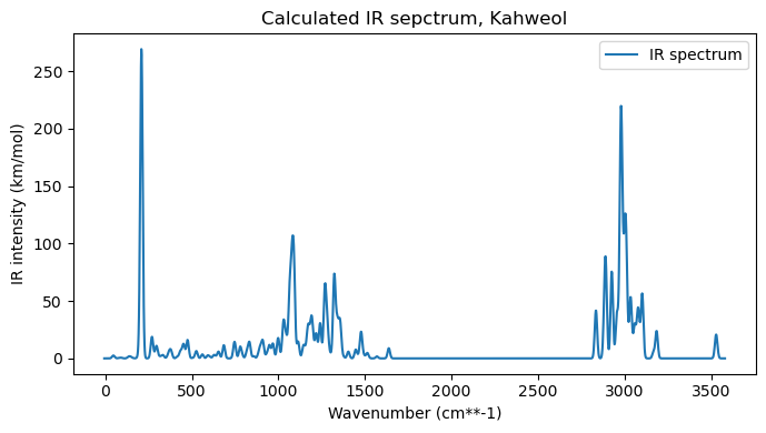
After adding the broadening, we can plot the spectrum and then animate a specific normal mode, selected based on its index.
wvn, ir = xtb_vibanalysis_drv.vib_frequencies, xtb_vibanalysis_drv.ir_intensities
wvng, irg = add_broadening(wvn, ir, line_profile='Gaussian', line_param=10, step=2)
# Plot the IR spectra
plt.figure(figsize=(7,4))

# Plot the IR spectrum
plt.plot(wvng, irg, label='IR spectrum')
plt.xlabel('Wavenumber (cm**-1)')
#plt.axis(xmin=3200, xmax=3500)
#plt.axis(ymin=-0.2, ymax=1.5)
plt.ylabel('IR intensity (km/mol)')
plt.title("Calculated IR sepctrum, Kahweol")
plt.legend()
plt.tight_layout(); plt.show()

# Visualize the vibrational mode
index = 64
print("\n\n\n       Normal mode %d: %.2f cm-1, %.2f km/mol." % (index,
                                                                xtb_vibanalysis_drv.vib_frequencies[index-1],
                                                                xtb_vibanalysis_drv.ir_intensities[index-1]))
normal_mode = get_normal_mode(xtb_opt_kahweol, xtb_vibanalysis_drv.normal_modes[index-1])
view = p3d.view(viewergrid=(1,1), width=600, height=300)
view.addModel(normal_mode, "xyz", {'vibrate': {'frames':10,'amplitude':0.75}})

view.setViewStyle({"style": "outline", "width": 0.05})
view.setStyle({"stick": {}, "sphere": {"scale": 0.25}})

view.animate({'loop': 'backAndForth'})
view.zoomTo()
view.show()
Normal mode 64: 1078.75 cm-1, 68.62 km/mol.
3Dmol.js failed to load for some reason. Please check your browser console for error messages.
To make a more interactive normal mode selection, we can create a slider using the ipywidgets Python module for Jupyter notebooks. To make use of the slider widget, we first need a routine which can plot the IR spectrum and animate a specific normal mode selected based on its index.
def vibration_viewer(index):
    freq = xtb_vibanalysis_drv.vib_frequencies[index-1]
    ir_intens = xtb_vibanalysis_drv.ir_intensities[index-1]
    # Plot the IR spectrum
    plt.figure(figsize=(7,4))
    plt.plot(wvng, irg)
    plt.plot(freq, ir_intens, 'o',  markersize=10)
    plt.xlabel('Wavenumber (cm**-1)')
    plt.ylabel('IR intensity (km/mol)')
    plt.title("Calculated IR sepctrum, Kahweol")
    plt.tight_layout(); plt.show()

    normal_mode = get_normal_mode(xtb_opt_kahweol, xtb_vibanalysis_drv.normal_modes[index-1])
    view = p3d.view(viewergrid=(1,1), width=600, height=300)
    view.addModel(normal_mode, "xyz", {'vibrate': {'frames':10,'amplitude':0.75}})
    view.setViewStyle({"style": "outline", "width": 0.05})
    view.setStyle({"stick": {}, "sphere": {"scale": 0.25}})
    view.animate({'loop': 'backAndForth'})
    view.zoomTo()
    view.show()
no_norm_modes = xtb_vibanalysis_drv.vib_frequencies.shape[0] # number of vibrational modes

# Note that the slider only works in a Jupyter notebook.
ipywidgets.interact(vibration_viewer,
                    index=ipywidgets.IntSlider(min=1, max=no_norm_modes, step=1, value=92))
<function __main__.vibration_viewer(index)>