Reduced particle densities

Reduced particle densities#

Consider an $N$ -electron system in a state represented by a general state vector that can be expressed as a linear combination of Slater determinants

| Ψ ⟩ = \sum_{n} c_{n} | Φ_{n} ⟩

The one- and two-particle particle reduced densities can be evaluated as expectation values of one- and two-particle operators, respectively, using the expressions for matrix elements. The resulting formulas will be expressions involving products of molecular orbitals from which we can identify one- and two-particle density matrices.

As an illustration, we will determine the one- and two-particle densities along the internuclear axis of carbon monoxide at the level of Hartree–Fock theory.

import matplotlib.pyplot as plt
import numpy as np
import veloxchem as vlx

mol_str = """
C        0.00000000    0.00000000    0.00000000
O        0.00000000    0.00000000    2.70000000
"""
molecule = vlx.Molecule.read_molecule_string(mol_str, units="au")
basis = vlx.MolecularBasis.read(molecule, "cc-pVDZ", ostream=None)

scf_drv = vlx.ScfRestrictedDriver()
scf_drv.ostream.mute()

scf_results = scf_drv.compute(molecule, basis)

C = scf_results["C_alpha"]
D = scf_results["D_alpha"] + scf_results["D_beta"]

norb = basis.get_dimensions_of_basis()
nocc = molecule.number_of_alpha_electrons()

print("Number of contracted basis functions:", norb)
print("Number of doubly occupied molecular orbitals:", nocc)

Number of contracted basis functions: 28
Number of doubly occupied molecular orbitals: 7

One-particle density#

Probabilistic interpretation#

The probability density of finding any one electron in an infinitesimal volume element at position $r$ regardless of the positions of other electrons is equal to

n (r) = N \int \dots \int Ψ^{†} (r, r_{2}, \dots, r_{N}) Ψ (r, r_{2}, \dots, r_{N}) d^{3} r_{2} \dots d^{3} r_{N}

Expectation values#

For a scalar one-electron operator in coordinate basis taking the form

\hat{Ω} = \sum_{i = 1}^{N} ω (r_{i})

the expectation value relates to the one-particle density according to

\begin{aligned} ⟨ \hat{Ω} ⟩ & = \int \dots \int Ψ^{†} (r_{1}, r_{2}, \dots, r_{N}) \hat{Ω} Ψ (r_{1}, r_{2}, \dots, r_{N}) d^{3} r_{1} d^{3} r_{2} \dots d^{3} r_{N} \\ = N \int ω (r) [\int \dots \int Ψ^{†} (r, r_{2}, \dots, r_{N}) Ψ (r, r_{2}, \dots, r_{N}) d^{3} r_{2} \dots d^{3} r_{N}] d^{3} r \\ = \int ω (r) n (r) d^{3} r \end{aligned}

One-particle density operator#

The one-particle density can be written as an expectation of a one-electron operator according to

n (r) = ⟨ Ψ | \hat{n} (r) | Ψ ⟩

where

\hat{n} (r) = \sum_{i = 1}^{N} δ (r - r_{i})

and $δ (r - r_{i})$ is the Dirac delta function.

After evaluation of this expectation value, the one-particle density matrix, $D$ , is identified from the expression

n (r) \equiv \sum_{p, q} D_{p q} ψ_{p}^{†} (r) ψ_{q} (r)

For a state represented by a single Slater determinant, the one-electron density becomes

n (r) = \sum_{i = 1}^{N} | ψ_{i} (r) |^{2}

where the summation run over the $N$ occupied spin orbitals. Consequently, the density matrix is in this case equal to the identity matrix in the occupied–occupied block and zero elsewhere.

For a restricted closed-shell state, we get

n (r) = 2 \sum_{i}^{occ} | ϕ_{i} (r) |^{2} = \sum_{p, q} D_{p q}^{MO} ϕ_{p}^{*} (r) ϕ_{q} (r)

where the summations runs over molecular orbitals (MOs) and the density matrix in the MO basis equals

\begin{array}{r} D^{MO} = (\begin{array}{c} 2 & \dots & 0 & 0 & \dots & 0 \\ ⋮ & ⋱ & ⋮ & ⋮ & ⋱ & ⋮ \\ 0 & \dots & 2 & 0 & \dots & 0 \\ 0 & \dots & 0 & 0 & \dots & 0 \\ ⋮ & ⋱ & ⋮ & ⋮ & ⋱ & ⋮ \\ 0 & \dots & 0 & 0 & \dots & 0 \end{array}) \end{array}

In the atomic orbital (AO) basis, we have

n (r) = \sum_{α, β} D_{α β}^{AO} χ_{α}^{*} (r) χ_{β} (r)

where

D_{α β}^{AO} = 2 \sum_{i}^{occ} c_{α i}^{*} c_{β i}

or, equivalently,

D^{AO} = C^{*} D^{MO} C^{T}

D_mo = np.zeros((norb, norb))

for i in range(nocc):
    D_mo[i, i] = 2.0

D_ao = np.einsum("ap, pq, bq -> ab", C, D_mo, C)

Test MO to AO transformation against the reference density matrix from VeloxChem.

np.testing.assert_allclose(D_ao, D, atol=1e-12)

Illustration#

The one-particle density is available in VeloxChem by means of the VisualizationDriver class. As indicated by the string argument “alpha” in the get_density method, the $α$ - and $β$ -spin densities can be determined individually, referring to the relation

n (r) = n^{α} (r) + n^{β} (r)

For a closed shell system, the two spin densities are equal and thus equal to half the total one-particle density.

Considering the one-particle density of CO, as calculated along the line intersecting both atoms:

vis_drv = vlx.VisualizationDriver()

# list of coordinates in units of Bohr
n = 2000
coords = np.zeros((n, 3))
z = np.linspace(-1, 4, n)
coords[:, 2] = z
one_part_den = vis_drv.get_density(coords, molecule, basis, scf_drv.density, "alpha")

fig = plt.figure(figsize=(12, 4))
plt.subplot(1, 2, 1)
plt.plot(z, one_part_den, lw=2, label=r"$n^\alpha(\mathbf{r})$")
plt.setp(plt.gca(), xlim=(-1, 4))
plt.legend()
plt.xlabel(r"Internuclear axis coordinate (Bohr)")
plt.ylabel(r"One-particle density (a.u.)")

plt.subplot(1, 2, 2)
plt.plot(z, one_part_den, lw=2, label=r"$n^\alpha(\mathbf{r})$")
plt.plot(z, one_part_den, "ko")
plt.grid(True)
plt.setp(plt.gca(), xlim=(-0.05, 0.05), ylim=(50, 62))
plt.legend()
plt.xlabel(r"Internuclear axis coordinate (Bohr)")
plt.ylabel(r"One-particle density (a.u.)")

plt.show()

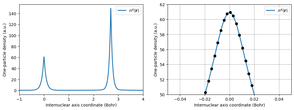
../../_images/b7a3ed7308a4f50b2397eb24bbd87e79be3ad19f43d08e418ae06ea1b5469033.png

The right figure panel is an enlargement of the one-particle density in the region of the carbon nucleus, illustrating the fact that $n (r)$ displays a cusp at any given nuclear position.

Two-particle density#

Probabilistic interpretation#

The probability density of finding any two electrons in separate infinitesimal volume elements at positions $r_{1}$ and $r_{2}$ regardless of the positions of other electrons is equal to

n (r_{1}, r_{2}) = N (N - 1) \int \dots \int Ψ^{†} (r_{1}, r_{2}, r_{3}, \dots, r_{N}) Ψ (r_{1}, r_{2}, r_{3}, \dots, r_{N}) d^{3} r_{3} \dots d^{3} r_{N}

Expectation values#

For a scalar two-electron operator in coordinate basis taking the form

\hat{Ω} = \sum_{j > i}^{N} ω (r_{i}, r_{j})

the expectation value relates to the one-particle density according to

\begin{aligned} ⟨ \hat{Ω} ⟩ & = \int \dots \int Ψ^{†} (r_{1}, \dots, r_{N}) \hat{Ω} Ψ (r_{1}, \dots, r_{N}) d^{3} r_{1} \dots d^{3} r_{N} \\ = \frac{N (N - 1)}{2} \int \int ω (r_{1}, r_{2}) [\int \dots \int Ψ^{†} (r_{1}, \dots, r_{N}) Ψ (r_{1}, \dots, r_{N}) d^{3} r_{3} \dots d^{3} r_{N}] d^{3} r_{1} d^{3} r_{2} \\ = \frac{1}{2} \int ω (r_{1}, r_{2}) n (r_{1}, r_{2}) d^{3} r_{1} d^{3} r_{2} \end{aligned}

Two-particle density operator#

The two-particle density can be written as an expectation of a two-electron operator according to

n (r, r^{'}) = ⟨ Ψ | \hat{n} (r, r^{'}) | Ψ ⟩

with

\hat{n} (r, r^{'}) = \sum_{i = 1}^{N} \sum_{j > i}^{N} [δ (r - r_{i}) δ (r^{'} - r_{j}) + δ (r - r_{j}) δ (r^{'} - r_{i})]

After evaluation of this expectation value, the two-particle density matrix, $D$ , is identified from the expression

n (r, r^{'}) \equiv \sum_{p, q, r, s} ψ_{p}^{†} (r) ψ_{q} (r) D_{p q r s} ψ_{r}^{†} (r^{'}) ψ_{s} (r^{'})

For a state represented by a single Slater determinant, the two-electron density becomes

n (r, r^{'}) = \sum_{i = 1}^{N} \sum_{j = 1}^{N} [| ψ_{i} (r) |^{2} | ψ_{j} (r^{'}) |^{2} - ψ_{i}^{†} (r) ψ_{j}^{†} (r^{'}) ψ_{j} (r) ψ_{i} (r^{'})]

where the summations run over the $N$ occupied spin orbitals.

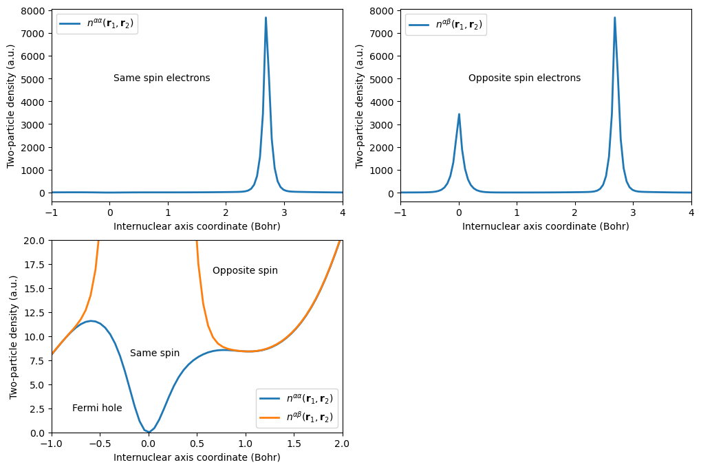
Illustration#

As indicated by the string arguments “alpha” and “beta” in the get_two_particle_density method, the spin densities can be determined individually, referring to the relation

n (r_{1}, r_{2}) = n^{α α} (r_{1}, r_{2}) + n^{α β} (r_{1}, r_{2}) + n^{β α} (r_{1}, r_{2}) + n^{β β} (r_{1}, r_{2})

For a closed shell system, we have

\begin{aligned} n^{α α} (r_{1}, r_{2}) & = n^{β β} (r_{1}, r_{2}) \\ n^{α β} (r_{1}, r_{2}) & = n^{β α} (r_{1}, r_{2}) \end{aligned}

We will determine the two-particle density for electron 1 being positioned at the carbon nucleus and electron 2 being positioned along the internuclear axis.

n = 100
origin = np.zeros((n, 3))
coords = np.zeros((n, 3))
z = np.linspace(-1, 4, n)
coords[:, 2] = z

two_part_den_aa = vis_drv.get_two_particle_density(
    origin, coords, molecule, basis, scf_drv.density, "alpha", "alpha"
)
two_part_den_ab = vis_drv.get_two_particle_density(
    origin, coords, molecule, basis, scf_drv.density, "alpha", "beta"
)

fig = plt.figure(figsize=(12, 8))
plt.subplot(2, 2, 1)
plt.plot(
    z, two_part_den_aa, lw=2, label=r"$n^{\alpha\alpha}(\mathbf{r}_1, \mathbf{r}_2)$"
)
plt.setp(plt.gca(), xlim=(-1, 4))
plt.legend()
plt.figtext(0.2, 0.75, r"Same spin electrons")
plt.xlabel(r"Internuclear axis coordinate (Bohr)")
plt.ylabel(r"Two-particle density (a.u.)")

plt.subplot(2, 2, 3)
plt.plot(
    z, two_part_den_aa, lw=2, label=r"$n^{\alpha\alpha}(\mathbf{r}_1, \mathbf{r}_2)$"
)
plt.plot(
    z, two_part_den_ab, lw=2, label=r"$n^{\alpha\beta}(\mathbf{r}_1, \mathbf{r}_2)$"
)
plt.setp(plt.gca(), xlim=(-1, 2), ylim=(0, 20))
plt.legend()
plt.figtext(0.22, 0.25, r"Same spin")
plt.figtext(0.15, 0.15, r"Fermi hole")
plt.figtext(0.32, 0.4, r"Opposite spin ")
plt.xlabel(r"Internuclear axis coordinate (Bohr)")
plt.ylabel(r"Two-particle density (a.u.)")

plt.subplot(2, 2, 2)
plt.plot(
    z, two_part_den_ab, lw=2, label=r"$n^{\alpha\beta}(\mathbf{r}_1, \mathbf{r}_2)$"
)
plt.setp(plt.gca(), xlim=(-1, 4))
plt.legend()
plt.figtext(0.63, 0.75, r"Opposite spin electrons")
plt.xlabel(r"Internuclear axis coordinate (Bohr)")
plt.ylabel(r"Two-particle density (a.u.)")

plt.show()

../../_images/a0e60220f16ef34776a663708e60b4d79362785d0f2791aa7b37601e0a0a9c41.png

Reduced particle densities

Contents

Reduced particle densities#

One-particle density#

Probabilistic interpretation#

Expectation values#

One-particle density operator#

Illustration#

Two-particle density#

Probabilistic interpretation#

Expectation values#

Two-particle density operator#

Illustration#