Rovibronic states#
The sum-over-states expressions for response functions are expressed in terms of the exact rovibronic eigenstates of the molecular Hamiltonian in the absence of external fields. These states are rarely available in practical calculations, where instead electronic states are employed. However, for a diatomic system, we can determine the rovibrational wave functions and the associated transition moments and energies.
Adopting the adiabatic Born–Oppenheimer approximation, the total molecular rovibronic wave function takes the form of a product
where \(K\) and \(k\) are indices identifying the electronic and rovibrational levels, respectively. For a diatomic system, the rovibrational wave function is in turn separated into its vibrational, \(\psi\), and rotational, \(\psi_\mathrm{r}\), components
where \(k\) is understood as a compound index uniquely identifying a given rotational level of a given vibrational state.
Rotational Schrödinger equation#
The Schrödinger equation for diatomic molecule with fixed bond length equals
or, equivalently,
where \(\hat{L}^2\) is the square of the total angular moment operator. The angles \(\theta\) and \(\phi\) describe the orientation of the diatomic molecule with respect to a laboratory-fixed coordinate system and \(\mu\) is the reduced mass defined as
The eigenfunctions to the total angular momentum operator are known to the the sperical harmonics, \(Y_J^M(\theta, \phi)\), and the associated rotational energies are given by
introducing the rotational constant \(B\). We note that rotational levels are \((2J+1)\)-fold degenerate.
Transitions between rotational levels are classified according to
Q-branch: when \(\Delta J = 0\)
R-branch: when \(\Delta J = +1\)
P-branch: when \(\Delta J = -1\)
Numerov’s method and the vibrational Schrödinger equation#
Numerov’s method can be employed to solve 1D differential equations using finite differences on a grid of points. It applies to a differential equation on the form
This method will be used to solve the vibrational part of the Schrödinger equation that for the lowest rotational level (\(J=0\)) takes the form
For notational convenience, we introduce \(x = (R - R_0)\) to arrive at
where
The values of the wave function in three equidistant points separated by \(h\) are related as
from which solutions are found by the algorithm
Guess the energy \(E_\mathrm{guess}\)
For \(E_\mathrm{guess}\), determine the classically allowed interval [\(x_a,x_b\)] inside \(V(x)\)
Pick two points \(x_\mathrm{min}\) and \(x_\mathrm{max}\) far into the classically forbidden region and impose the wave function to be zero at these points
Determine iteratively the wave functions inside the interval \([x_\mathrm{min}, x_\mathrm{max}]\):
If \(\psi(x_a)<\epsilon\) and \(\psi(x_b)<\epsilon\), accept the wave function
If not, renew the energy guess
Numerov’s method in VeloxChem#
import matplotlib.pyplot as plt
import numpy as np
import veloxchem as vlx
We will use HCl as an example.
mol_str = """
Cl   0.0     0.0   0.0
H    1.274   0.0   0.0
"""

molecule = vlx.Molecule.read_molecule_string(mol_str, units="angstrom")

basis_set_label = "6-31+G"
basis = vlx.MolecularBasis.read(molecule, basis_set_label)

scf_settings = {"conv_thresh": 1.0e-6}
method_settings = {"xcfun": "b3lyp", "grid_level": 4}
The following settings are available for the Numerov solver in VeloxChem.
num_drv = vlx.NumerovDriver()
num_drv.print_keywords()
                ==========================================================================================
                  @numerov
                ------------------------------------------------------------------------------------------
                  pec_displacements  sequence    PEC scanning range [bohr]
                  pec_potential      string      potential type for fitting
                  reduced_mass       float       reduced mass of the molecule
                  el_transition      boolean     include an electronic transition
                  final_el_state     integer     final state of the electronic transition
                  exc_conv_thresh    float       excited state calculation threshold
                  n_vib_states       integer     number of vibrational states to be resolved
                  temp               float       temperature in Kelvin
                  n_rot_states       integer     number of rotational states to be resolved
                  conv_thresh        float       convergence threshold for vibronic energies
                  max_iter           integer     max. iteration number per vibronic state
                  n_margin           float       negative margin of the grid [bohr]
                  p_margin           float       positive margin of the grid [bohr]
                  steps_per_au       integer     number of grid points per Bohr radius
                ==========================================================================================
We will determine the potential on an interval of
numerov_settings = {
    "n_vib_states": 4,
    "pec_displacements": "-0.3 - 0.9 (0.2)",
    "el_transition": "no",
    "pec_potential": "morse",
    "n_rot_states": 10,
}
num_drv.update_settings(numerov_settings, scf_settings, method_settings)
num_results = num_drv.compute(molecule, basis)
                                           Potential Energy Curve Driver Setup
                                          =====================================

                              Number of Geometries          : 7
                              Wave Function Model           : Spin-Restricted Kohn-Sham
                              SCF Convergece Threshold      : 1.0e-06
                              DFT Functional                : B3LYP
                              Molecular Grid Level          : 4
*** Geometry 1/7: Initial state converged
*** Geometry 2/7: Initial state converged
*** Geometry 3/7: Initial state converged
*** Geometry 4/7: Initial state converged
*** Geometry 5/7: Initial state converged
*** Geometry 6/7: Initial state converged
*** Geometry 7/7: Initial state converged
               Potential Energy Curve Information
               ----------------------------------
                                               rel. GS energy
               Bond distance:     1.1152 angs      0.85540 eV
               Bond distance:     1.2211 angs      0.16191 eV
               Bond distance:     1.3269 angs      0.00000 eV
               Bond distance:     1.4328 angs      0.13406 eV
               Bond distance:     1.5386 angs      0.42849 eV
               Bond distance:     1.6444 angs      0.80534 eV
               Bond distance:     1.7503 angs      1.21628 eV
                                                   Numerov Driver Setup
                                                  ======================

                                         Number of Vibrational States : 4
                                         Energy Convergence Threshold : 1.0e-12
                                         Max. Number of Iterations    : 1000
                                         Grid Points per Bohr Radius  : 500
                                         Margin right of scanned PEC  : 1.50
                                         Margin left of scanned PEC   : 0.50
*** Vibronic state 0 converged in 109 iterations
*** Vibronic state 1 converged in 178 iterations
*** Vibronic state 2 converged in 160 iterations
*** Vibronic state 3 converged in 144 iterations
*** All vibronic states converged for the initial electronic state
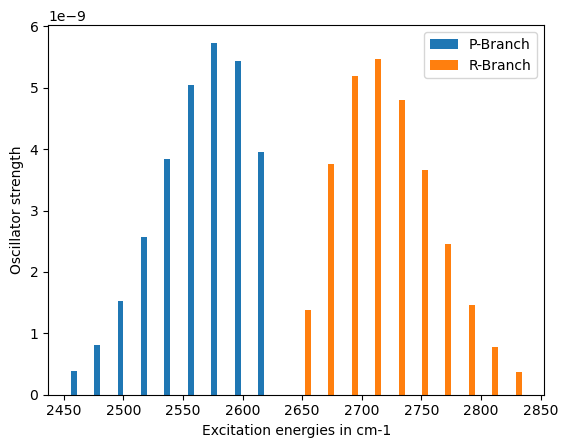
               Rovibronic IR Spectrum
               ----------------------
                           Excitation energy    Oscillator strength
               P Branch
                                2615.49 cm-1            3.94747e-09
                                2595.85 cm-1            5.44302e-09
                                2576.21 cm-1            5.73425e-09
                                2556.57 cm-1            5.04621e-09
                                2536.93 cm-1            3.83968e-09
                                2517.28 cm-1            2.56958e-09
                                2497.64 cm-1            1.52708e-09
                                2478.00 cm-1            8.10792e-10
                                2458.36 cm-1            3.86134e-10
               Q Branch
                                2635.13 cm-1            5.86085e-08
               R Branch
                                2654.77 cm-1            1.37859e-09
                                2674.42 cm-1            3.76177e-09
                                2694.06 cm-1            5.18696e-09
                                2713.70 cm-1            5.46448e-09
                                2733.34 cm-1            4.80881e-09
                                2752.98 cm-1            3.65905e-09
                                2772.62 cm-1            2.44870e-09
                                2792.26 cm-1            1.45524e-09
                                2811.91 cm-1            7.72649e-10
                                2831.55 cm-1            3.67969e-10
The results are stored in a dictionary.
print(num_results.keys())
dict_keys(['grid', 'potential', 'psi', 'vib_levels', 'excitation_energies', 'oscillator_strengths'])
grid = num_results["grid"]
potential = num_results["potential"]

vib_psi2 = num_results["psi"] ** 2
vib_energies = num_results["vib_levels"]

exc = num_results["excitation_energies"]
osc = num_results["oscillator_strengths"]
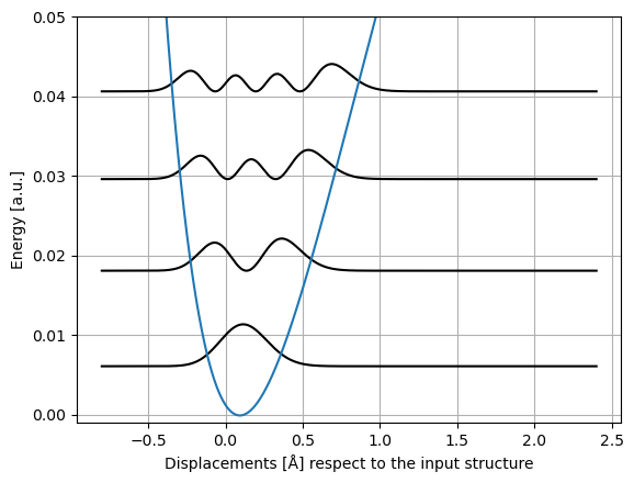
The vibrational levels can be plotted against the potential energy curve.
fig, ax1 = plt.subplots()

for energy, psi2 in zip(vib_energies, vib_psi2):
    ax1.plot(grid, energy + psi2, "k")

ax = plt.subplot()
ax.plot(grid, potential)
ax.set_ylim(-0.001, 0.05)
ax.set_xlabel("Displacements [Å] respect to the input structure")
ax.set_ylabel("Energy [a.u.]")

plt.grid(True)

plt.show()
Rovibrational spectra#
Once we have the vibrational wave functions we can calculate the dipole transition moments
where \(\mu(R)\) is the electronic dipole moment at internuclear separation distance \(R\).
Only the first transition dipole moment (corresponding to the Q-branch) is relevant and the rest are negligible. We will obtain the fine structure by deriving the rotational excited states for the R and P branches.
Applying the rotational selection rules derived before for the rigid rotor, we get the P-branch (\(\Delta J = -1\))
and the R-branch (\(\Delta J = +1\))
where
VeloxChem takes care of the spectra and the branches storing the data on the keys: excitation_energies and oscillator_strengths.
As well, computes the dipole moment for every point of the potential energy curve
ax1 = plt.bar(exc["P"], osc["P"], width=5.0, label="P-Branch")
ax2 = plt.bar(exc["R"], osc["R"], width=5.0, label="R-Branch")
plt.xlabel("Excitation energies in cm-1")
plt.ylabel("Oscillator strength")
plt.legend()

plt.show()
Vibronic transitions#
In this case, we want to consider the transition dipole moments between rovibrational states in different electronic states. The expression for the transition dipole integral will in this case involve the ground, \(|0\rangle\), and final, \(|F\rangle\), electronic states.
Expanding the electronic transition moment in a Taylor series about the equilibrium distance of the ground electronic state, we get
Truncating this expansion to first and second order are known as the Frank–Condon and Herzberg–Teller approximations, respectively. We will here adopt the former.
num_drv = vlx.NumerovDriver()

numerov_settings = {
    "n_vib_states": 3,
    "pec_displacements": "-0.3 - 0.9 (0.2)",
    "el_transition": "yes",
    "final_el_state": 2,
    "pec_potential": "morse",
}
num_drv.update_settings(numerov_settings, scf_settings, method_settings)
num_results = num_drv.compute(molecule, basis)
                                           Potential Energy Curve Driver Setup
                                          =====================================

                              Number of Geometries          : 7
                              Wave Function Model           : Spin-Restricted Kohn-Sham
                              SCF Convergece Threshold      : 1.0e-06
                              DFT Functional                : B3LYP
                              Molecular Grid Level          : 4
                              Targeted Exicted State        : 2
                              Excited State Threshold       : 1.0e-04
*** Geometry 1/7: Initial state converged, Final state converged
*** Geometry 2/7: Initial state converged, Final state converged
*** Geometry 3/7: Initial state converged, Final state converged
*** Geometry 4/7: Initial state converged, Final state converged
*** Geometry 5/7: Initial state converged, Final state converged
*** Geometry 6/7: Initial state converged, Final state converged
*** Geometry 7/7: Initial state converged, Final state converged
               Potential Energy Curve Information
               ----------------------------------
                                               rel. GS energy  rel. ES energy
               Bond distance:     1.1152 angs      0.85540 eV     11.00371 eV
               Bond distance:     1.2211 angs      0.16191 eV     10.18856 eV
               Bond distance:     1.3269 angs      0.00000 eV      9.77836 eV
               Bond distance:     1.4328 angs      0.13406 eV      9.68682 eV
               Bond distance:     1.5386 angs      0.42849 eV      9.83574 eV
               Bond distance:     1.6444 angs      0.80534 eV     10.11225 eV
               Bond distance:     1.7503 angs      1.21628 eV     10.28673 eV
                                                   Numerov Driver Setup
                                                  ======================

                                         Number of Vibrational States : 3
                                         Energy Convergence Threshold : 1.0e-12
                                         Max. Number of Iterations    : 1000
                                         Grid Points per Bohr Radius  : 500
                                         Margin right of scanned PEC  : 1.50
                                         Margin left of scanned PEC   : 0.50
*** Vibronic state 0 converged in 104 iterations
*** Vibronic state 1 converged in 175 iterations
*** Vibronic state 2 converged in 168 iterations
*** All vibronic states converged for the initial electronic state
*** Vibronic state 0 converged in 111 iterations
*** Vibronic state 1 converged in 139 iterations
*** Vibronic state 2 converged in 158 iterations
*** All vibronic states converged for the final electronic state
               UV/vis Absorption/Emission Spectrum
               -----------------------------------
                             Excitation energy    Oscillator strength
               Absorption
                                 78431.04 cm-1            2.62970e-01
                                 80560.28 cm-1            5.18422e-02
                                 82592.21 cm-1            3.98800e-03
               Emission
                                 78431.04 cm-1            2.62970e-01
                                 75795.91 cm-1            1.01134e-01
                                 73268.40 cm-1            6.47555e-03
print(num_results.keys())
dict_keys(['grid', 'i_potential', 'i_psi', 'i_vib_levels', 'f_potential', 'f_psi', 'f_vib_levels', 'excitation_energies', 'oscillator_strengths'])
grid = num_results["grid"]

dE_elec = np.min(num_drv.pec_energies["f"]) - np.min(num_drv.pec_energies["i"])

gs_potential = num_results["i_potential"]
gs_vib_psi2 = num_results["i_psi"] ** 2
gs_vib_energies = num_results["i_vib_levels"]

es_potential = num_results["f_potential"]
es_vib_psi2 = num_results["f_psi"] ** 2
es_vib_energies = num_results["f_vib_levels"]

exc = num_results["excitation_energies"]
osc = num_results["oscillator_strengths"]
displacements = num_drv.pec_displacements
gs_energies = num_drv.pec_energies["i"]
es_energies = num_drv.pec_energies["f"]

delta_E = np.min(es_energies) - np.min(gs_energies)
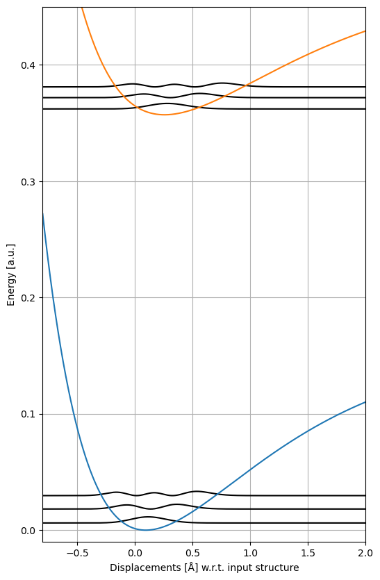
The vibrational levels can be then plotted against the potential energy curves:
fig, ax1 = plt.subplots(figsize=(6, 10))

for energy, psi2 in zip(gs_vib_energies, gs_vib_psi2):
    ax1.plot(grid, energy + psi2, "k")

for energy, psi2 in zip(es_vib_energies, es_vib_psi2):
    ax1.plot(grid, delta_E + energy + psi2, "k")

ax = plt.subplot()
ax.plot(grid, gs_potential)
ax.plot(grid, es_potential + delta_E)
ax.set_xlim(-0.8, 2.0)
ax.set_ylim(-0.01, 0.45)
ax.grid(True)
ax.set_xlabel("Displacements [Å] w.r.t. input structure")
ax.set_ylabel("Energy [a.u.]")

plt.show()
Now we can just plot the spectrum by representing the results from the driver:
plt.bar(exc["emission"], osc["emission"], width=500.0, label="emission")
plt.bar(exc["absorption"], osc["absorption"], width=500.0, label="absorption")

plt.legend()
plt.xlabel("Excitation energies in cm-1")
plt.ylabel("Oscillator strength")

plt.show()
User defined potential#
As an alternative to the automatized determination of potential energy curves and transition moments, these may be instead be determined separately, perhaps with a highly accurate post-Hartree–Fock approach. The method read_pec_data is then used.
As a simple illustration, we will use two harmonic potentials and transition moment that is independent of nuclear displacements.
num_drv = vlx.NumerovDriver()
x = np.arange(-0.7, 2.01, 0.1)

delta_E = 0.2

bond_lengths = x + 2.0
gs_energies = 0.75 * x**2
es_energies = 0.5 * (x - 0.35) ** 2 + delta_E

tmom = [0, 0, 1.0]
trans_moments = [tmom for displacement in x]
num_drv.read_pec_data(bond_lengths, trans_moments, gs_energies, es_energies)

num_drv.set_reduced_mass(1.0)

numerov_settings = {
    "n_vib_states": 10,
    "el_transition": "yes",
    "final_el_state": 1,
    "pec_potential": "harmonic",
}
num_drv.update_settings(numerov_settings, scf_settings, method_settings)
num_results = num_drv.compute()
                                                   Numerov Driver Setup
                                                  ======================

                                         Number of Vibrational States : 10
                                         Energy Convergence Threshold : 1.0e-12
                                         Max. Number of Iterations    : 1000
                                         Grid Points per Bohr Radius  : 500
                                         Margin right of scanned PEC  : 1.50
                                         Margin left of scanned PEC   : 0.50
*** Vibronic state 0 converged in 120 iterations
*** Vibronic state 1 converged in 194 iterations
*** Vibronic state 2 converged in 193 iterations
*** Vibronic state 3 converged in 190 iterations
*** Vibronic state 4 converged in 191 iterations
*** Vibronic state 5 converged in 187 iterations
*** Vibronic state 6 converged in 188 iterations
*** Vibronic state 7 converged in 194 iterations
*** Vibronic state 8 converged in 195 iterations
*** Vibronic state 9 converged in 200 iterations
*** All vibronic states converged for the initial electronic state
*** Vibronic state 0 converged in 103 iterations
*** Vibronic state 1 converged in 172 iterations
*** Vibronic state 2 converged in 167 iterations
*** Vibronic state 3 converged in 170 iterations
*** Vibronic state 4 converged in 170 iterations
*** Vibronic state 5 converged in 167 iterations
*** Vibronic state 6 converged in 172 iterations
*** Vibronic state 7 converged in 173 iterations
*** Vibronic state 8 converged in 171 iterations
*** Vibronic state 9 converged in 167 iterations
*** All vibronic states converged for the final electronic state
UV/vis Absorption/Emission Spectrum
-----------------------------------
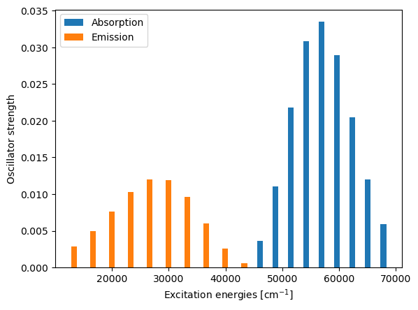
Excitation energy Oscillator strength
Absorption
43314.88 cm-1 5.67445e-04
46035.10 cm-1 3.61293e-03
48755.33 cm-1 1.10780e-02
51475.56 cm-1 2.17810e-02
54195.79 cm-1 3.08405e-02
56916.02 cm-1 3.34778e-02
59636.25 cm-1 2.89534e-02
62356.48 cm-1 2.04635e-02
65076.70 cm-1 1.20261e-02
67796.93 cm-1 5.94669e-03
Emission
43314.88 cm-1 5.67445e-04
39983.29 cm-1 2.56212e-03
36651.70 cm-1 5.98373e-03
33320.12 cm-1 9.60179e-03
29988.53 cm-1 1.18635e-02
26656.95 cm-1 1.19878e-02
23325.36 cm-1 1.02682e-02
19993.77 cm-1 7.61992e-03
16662.19 cm-1 4.95672e-03
13330.60 cm-1 2.83167e-03
Retrieving results from the calculation.
grid = num_results["grid"]

gs_potential = num_results["i_potential"]
gs_psi2 = num_results["i_psi"] ** 2
gs_vib_energies = num_results["i_vib_levels"]

es_potential = num_results["f_potential"]
es_psi2 = num_results["f_psi"] ** 2
es_vib_energies = num_results["f_vib_levels"]

exc = num_results["excitation_energies"]
osc = num_results["oscillator_strengths"]
Plotting potentials and vibrational wave functions.
fig, ax1 = plt.subplots(figsize=(6, 10))

for energy, psi2 in zip(gs_vib_energies, gs_psi2):
    ax1.plot(grid, energy + psi2, "k")

for energy, psi2 in zip(es_vib_energies, es_psi2):
    ax1.plot(grid, delta_E + energy + psi2, "k")

ax = plt.subplot()

ax.plot(grid, gs_potential)
ax.plot(grid, es_potential + delta_E)

ax.set_xlim(-1.5, 2.2)
ax.set_ylim(-0.01, 0.35)

ax.grid(True)

plt.show()
Plotting the vibronic absorption and emission spectra.
plt.bar(exc["absorption"], osc["absorption"], width=1000.0, label="Absorption")
plt.bar(exc["emission"], osc["emission"], width=1000.0, label="Emission")

plt.legend()
plt.xlabel(r"Excitation energies [cm$^{-1}$]")
plt.ylabel("Oscillator strength")

plt.show()