Dispersion interactions

Long-range interaction energy

The interaction energy between two molecular systems \(A\) and \(B\) is given by

\[ \Delta E = E_\mathrm{AB} - E_\mathrm{A} - E_\mathrm{B} \]

For charge neutral, nonpolar, systems separated by a sufficiently large distance \(R\) this interaction energy is known as dispersion (or van der Waals) energy.

Dispersion and correlation

The prototypical system exemplifying dispersion interactions is the He dimer for which the interaction energy equals

\[ \Delta E(R) = E_\mathrm{dimer} - 2E_\mathrm{He} \]

We will determine this interaction energy with respect to the interatomic separation distance at the Hartree–Fock and MP2 levels of theory.

import matplotlib.pyplot as plt
import numpy as np
import scipy
import veloxchem as vlx

au2ang = 0.529177

atom_xyz = """1
He atom
He    0.000000000000        0.000000000000        0.000000000000
"""

dimer_xyz = """2
He dimer
He    0.000000000000        0.000000000000        0.000000000000
He    0.000000000000        0.000000000000        dimer_separation
"""

atom = vlx.Molecule.read_xyz_string(atom_xyz)
atom_basis = vlx.MolecularBasis.read(atom, "aug-cc-pvtz", ostream=None)

dimer = vlx.Molecule.read_xyz_string(dimer_xyz.replace("dimer_separation", "5.0"))
dimer_basis = vlx.MolecularBasis.read(dimer, "aug-cc-pvtz", ostream=None)

Determine the atomic energies the HF and MP2 levels of theory.

scf_drv = vlx.ScfRestrictedDriver()
mp2_drv = vlx.mp2driver.Mp2Driver()
scf_drv.ostream.mute()
mp2_drv.ostream.mute()

scf_results = scf_drv.compute(atom, atom_basis)
hf_atom_energy = scf_drv.get_scf_energy()

mp2_results = mp2_drv.compute(atom, atom_basis, scf_drv.mol_orbs)
mp2_atom_energy = hf_atom_energy + mp2_results["mp2_energy"]

Determine the dimer energies over a range of interatomic separation distance.

distances = np.linspace(2.75, 5.0, 10)
hf_dimer_energies = []
mp2_dimer_energies = []

for dist in distances:

    dimer = vlx.Molecule.read_xyz_string(
        dimer_xyz.replace("dimer_separation", str(dist))
    )

    scf_results = scf_drv.compute(dimer, dimer_basis)
    hf_dimer_energies.append(scf_drv.get_scf_energy())
    mp2_results = mp2_drv.compute(dimer, dimer_basis, scf_drv.mol_orbs)
    mp2_dimer_energies.append(scf_drv.get_scf_energy() + mp2_results["mp2_energy"])

hf_dimer_energies = np.array(hf_dimer_energies)
mp2_dimer_energies = np.array(mp2_dimer_energies)

Plot the interaction energies in units of micro-Hartree.

hf_interaction_energies = hf_dimer_energies - 2 * hf_atom_energy
mp2_interaction_energies = mp2_dimer_energies - 2 * mp2_atom_energy

R = np.linspace(2.75, 5.0, 1000)

plt.figure(figsize=(7, 5))
x, y = distances, hf_interaction_energies * 1e6
f = scipy.interpolate.interp1d(x, y, kind="cubic")
plt.plot(R, f(R), "g-", label="HF")
plt.plot(x, y, "go")

x, y = distances, mp2_interaction_energies * 1e6
f = scipy.interpolate.interp1d(x, y, kind="cubic")
plt.plot(R, f(R), "b-", label="MP2")
plt.plot(x, y, "bs")

plt.xlabel("He-He distance (Å)")
plt.ylabel(r"Interaction energy ($\mu E_h$)")
plt.ylim(-30, 50)
plt.legend()
plt.grid(True)
plt.show()

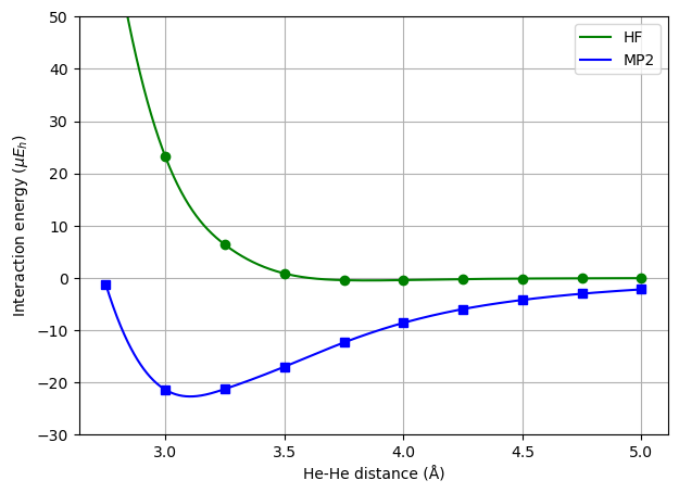
The failure of the HF method to describe the minimum of the potential energy curve for the helium dimer is due to the lack of correlation. More specifically, let us consider a system setup where the \(z\)-axis is chosen as the internuclear axis and the helium atoms are placed at \(z = 0\) and \(z=R_0\), respectively (see the inset in the figure below). We will then be concerned with the two-particle density, \(n(\mathbf{r}_1, \mathbf{r}_2)\), at coordinates

\[\begin{align*} \mathbf{r}_1 & = (d, 0,0) \\ \mathbf{r}_2 & = (d \cos\theta, d \sin\theta,R_0) \\ \end{align*}\]

At the HF level of theory, the two-particle density will be independent of the angle \(\theta\) whereas this is not the case when electron correlation is accounted for. The MP2 density shows a maximum when the two electrons are positioned as far apart as possible, or in other words as \(\theta = 180^\circ\).

This asymmetry in the two-particle density is referred to as fluctuating induced dipoles, or instantaneous dipole–dipole interactions, and it is the source origin of the weakly attractive van der Waals energies.

Dispersion by perturbation theory

The long-range interaction energy between two randomly oriented molecules \(A\) and \(B\) is given by the Casimir–Polder potential

\[\begin{eqnarray*} \Delta E(R) & = & - \frac{\hbar}{\pi R^6} \int_{0}^{\infty} \overline{\alpha}_A(i\omega^I) \overline{\alpha}_B(i\omega^I) e^{-2\omega^I R/c} \\ \nonumber && \quad \times \left[ 3 + 6 \frac{\omega^I R}{c} + 5 \left(\frac{\omega^I R}{c}\right)^2 + 2 \left(\frac{\omega^I R}{c}\right)^3 + \left(\frac{\omega^I R}{c}\right)^4 \right] d\omega^I \end{eqnarray*}\]

where \(R\) is the intermolecular separation, \(c\) is the speed of light, and \(\overline{\alpha}_A(i\omega^I)\) is the isotropic average of the electric dipole polarizability tensor of molecule \(A\) evaluated at a purely imaginary frequency. The molecules are here considered to be polarizable entities. Additional contributions to the energy will arise from higher-order electric multipole interactions as well as magnetic interactions.

The interaction energy is often expressed in terms of dispersion coefficients \(C_m\), where \(m = 6, 8, 10, \ldots\), and long-range coefficients \(K_n\), where \(n = 7, 9, 11, \ldots\), so that, in the van der Waals region, we have

\[\begin{equation*} \Delta E(R) = -\frac{C_6}{R^6} -\frac{C_8}{R^8} -\frac{C_{10}}{R^{10}} - \cdots \end{equation*}\]

and, at very large intermolecular separation, we have

\[\begin{equation*} \Delta E(R) = -\frac{K_7}{R^7} -\frac{K_9}{R^9} -\frac{K_{11}}{R^{11}} - \cdots \end{equation*}\]

The reason for the deviation of the interaction energy at large \(R\) from a \(1/R^6\) dependence, as given by London–van der Waals dispersion theory, is the finite speed of the photons mediating the electromagnetic interaction, or, equivalently, retardation.

The leading dispersion coefficient is given by

\[\begin{equation*} C_6 = \frac{3\hbar}{\pi} \int_{0}^{\infty} \overline{\alpha}_A(i\omega) \overline{\alpha}_B(i\omega) d\omega \end{equation*}\]

c6_drv = vlx.C6Driver()
c6_drv.ostream.mute()
scf_results = scf_drv.compute(atom, atom_basis)
c6_results = c6_drv.compute(atom, atom_basis, scf_results)

hf_c6 = c6_results["c6"]

Based on Hartree–Fock data and with access to the \(C_6\) dispersion coefficient, a much more realistic potential energy curve can be constructed as follows

\[ \Delta E(R) = \Delta E^\mathrm{HF}(R) - \frac{C_6}{R^6} \]

where the first and second term contribute the repulsive and attractive parts of the potential, respectively.

plt.figure(figsize=(7, 5))

# Reference data at FCI level
plt.axvline(5.6 * au2ang, color="navy")
plt.axhline(-28.76, color="navy")
plt.text(3.01, -34, "FCI reference")

x, y = distances, hf_interaction_energies * 1e6
f = scipy.interpolate.interp1d(x, y, kind="cubic")
plt.plot(R, f(R), "g-", label="HF")
plt.plot(x, y, "go")

x, y = distances, mp2_interaction_energies * 1e6
f = scipy.interpolate.interp1d(x, y, kind="cubic")
plt.plot(R, f(R), "b-", label="MP2")
plt.plot(x, y, "bs")

x, y = distances, (hf_interaction_energies - hf_c6 / (distances / au2ang) ** 6) * 1e6
f = scipy.interpolate.interp1d(x, y, kind="cubic")
plt.plot(R, f(R), "m-", label="HF + C6")
plt.plot(x, y, "m^")

plt.xlabel("He-He distance (Å)")
plt.ylabel(r"Interaction energy ($\mu E_h$)")
plt.ylim(-40, 50)
plt.legend()
plt.grid(True)
plt.show()

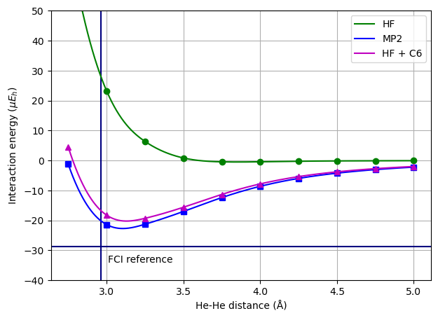
A FCI reference value for the binding energy, 29 \(\mu E_h\), and equilibrium distance, 2.96 Å [VvLvD90], is depicted in the figure as the crossing point of the vertical and horizontal lines. Both the MP2 and the dispersion-corrected HF minima are quite close to this FCI reference point.

It has become a standard procedure to adopt a similar approach to add dispersion corrections to DFT potentials as standard functionals do not offer an inclusion of dispersion interactions. This can be very important when performing molecular structure optimizations of systems with nonbonded interactions.