Rayleigh–Schrödinger perturbation theory

Rayleigh–Schrödinger perturbation theory#

Since the Hartree–Fock state in many cases approximates the exact electronic ground state wave function quite well, it is natural to use perturbation theory as a means to improve the description. The starting point it to divide the Hamiltonian into two parts

\hat{H} = {\hat{H}}_{0} + \hat{V}

where ${\hat{H}}_{0}$ is some zeroth-order Hamiltonian and $\hat{V}$ is the perturbation. The orthonormal eigenstates of ${\hat{H}}_{0}$ are assumed to be known

{\hat{H}}_{0} | Φ_{n} ⟩ = E_{n} | Φ_{n} ⟩

The exact ground state is a solution to the time-independent Schrödinger equation

\hat{H} | Ψ ⟩ = E | Ψ ⟩

where $| Ψ ⟩$ and $E$ are expanded in orders of $\hat{V}$

\begin{aligned} | Ψ ⟩ & = \sum_{k = 0}^{\infty} | Ψ^{(k)} ⟩ \\ E & = \sum_{k = 0}^{\infty} E^{(k)} \end{aligned}

Such an order-by-order procedure may converge given that ${\hat{H}}_{0}$ includes the main features of $\hat{H}$ , and that $\hat{V}$ in some sense is significantly smaller than ${\hat{H}}_{0}$ . We get

({\hat{H}}_{0} + \hat{V}) \sum_{k = 0}^{\infty} | Ψ^{(k)} ⟩ = \sum_{k, l} E^{(k)} | Ψ^{(l)} ⟩

Collecting terms to order $m$ gives us the master equation of Rayleigh–Schrödinger pertubation theory (RSPT)

({\hat{H}}_{0} - E^{(0)}) | Ψ^{(m)} ⟩ = - \hat{V} | Ψ^{(m - 1)} ⟩ + \sum_{k = 1}^{m} E^{(k)} | Ψ^{(m - k)} ⟩

Solving the RSPT master equation#

To zeroth order, we get

({\hat{H}}_{0} - E^{(0)}) | Ψ^{(0)} ⟩ = 0

resulting in

| Ψ^{(0)} ⟩ = | Φ_{0} ⟩; E^{(0)} = E_{0}

We note that the component of $| Φ_{0} ⟩$ in higher-order corrections $| Ψ^{(m)} ⟩$ becomes undetermined since

({\hat{H}}_{0} - E^{(0)}) [| Ψ^{(m)} ⟩ + c_{0}^{(m)} | Φ_{0} ⟩] = ({\hat{H}}_{0} - E^{(0)}) | Ψ^{(m)} ⟩

We will choose $c_{0}^{(m)} = 0$ such that $⟨ Ψ^{(0)} | Ψ^{(m)} ⟩ = 0$ for $m > 0$ . This corresponds to a choice of intermediate normalization

\begin{aligned} ⟨ Ψ^{(0)} | Ψ ⟩ & = \sum_{k = 0}^{\infty} ⟨ Ψ^{(0)} | Ψ^{(k)} ⟩ = ⟨ Ψ^{(0)} | Ψ^{(0)} ⟩ = 1 \end{aligned}

With this choice made, the energy corrections are easily obtained from the RSPT master equation by a projection with $⟨ Ψ^{(0)} |$ :

E^{(m)} = ⟨ Ψ^{(0)} | \hat{V} | Ψ^{(m - 1)} ⟩; m > 0

Wave function corrections are obtained from the RSPT master equation by multiplying with the inverse and projecting out the zeroth-order solution in accordance with choice of intermediate normalization

| Ψ^{(m)} ⟩ = - \hat{P} ({\hat{H}}_{0} - E^{(0)})^{- 1} \hat{P} [\hat{V} | Ψ^{(m - 1)} ⟩ - \sum_{k = 1}^{m - 1} E^{(k)} | Ψ^{(m - k)} ⟩]

where

\hat{P} = \hat{I} - | Ψ^{(0)} ⟩ ⟨ Ψ^{(0)} |

Numerical illustration#

Let us set up a ten-states model of a system. This setup includes defining a diagonal zeroth-order Hamiltonian matrix, $H_{0}$ , and a comparatively smaller perturbation matrix, $V$ , without coupling between the ground and first excited state. The state energy separation in the unperturbed system is customizable.

import numpy as np

np.set_printoptions(precision=4, suppress=True, linewidth=132)


def setup_system(energy_separation=0.5, verbose=False, n=10):

    E_0 = 1.5
    Phi_0 = np.zeros(n)
    Phi_0[0] = 1

    H_0_diag = np.arange(E_0, E_0 + energy_separation * n, energy_separation)
    H_0 = np.diag(H_0_diag)

    np.random.seed(20220526)
    V = -0.1 * np.diag(np.random.rand(n) * 0.1)
    for i in range(2, n):
        V[i - 2 : i, i] = np.random.rand(2) * 0.25
    V = V + V.T

    H = H_0 + V

    eigval, _ = np.linalg.eigh(H)
    E_exact = eigval.min()

    # M = P * (H_0 - E_0)^{-1} * P
    M_diag = H_0_diag - E_0
    M_diag[0] = 1
    M = np.diag(1 / M_diag)
    M[0, 0] = 0

    E = [E_0]
    Psi = [Phi_0]

    if verbose:
        print(H)

    return E_exact, E, Psi, V, M

For a given system, the RSPT equations are solved to determine the energy up to a given order. In a first example, we consider a system where the separation energy is 0.50 and equals twice the maximum perturbation energy of 0.25.

E_exact, E, Psi, V, M = setup_system(energy_separation=0.5, verbose=True, n=10)

[[1.4931 0.     0.1577 0.     0.     0.     0.     0.     0.     0.    ]
 [0.     1.9948 0.2499 0.0431 0.     0.     0.     0.     0.     0.    ]
 [0.1577 0.2499 2.4836 0.1796 0.2426 0.     0.     0.     0.     0.    ]
 [0.     0.0431 0.1796 2.9848 0.1341 0.2125 0.     0.     0.     0.    ]
 [0.     0.     0.2426 0.1341 3.4843 0.2393 0.0742 0.     0.     0.    ]
 [0.     0.     0.     0.2125 0.2393 3.9982 0.1831 0.0795 0.     0.    ]
 [0.     0.     0.     0.     0.0742 0.1831 4.492  0.2116 0.2425 0.    ]
 [0.     0.     0.     0.     0.     0.0795 0.2116 4.9965 0.1532 0.0945]
 [0.     0.     0.     0.     0.     0.     0.2425 0.1532 5.4865 0.2328]
 [0.     0.     0.     0.     0.     0.     0.     0.0945 0.2328 5.9925]]

def rspt_solver(E_exact, E, Psi, V, M, verbose=False):

    error = [E[0] - E_exact]

    if verbose:
        print(" n   RSPT energy    Error")
        print(f" 0 {E[0]:12.8f} {error[0]:14.8f}")

    for m in range(1, 10):

        E.append(np.einsum("i,ij,j", Psi[0], V, Psi[m - 1]))
        error.append(np.array(E).sum() - E_exact)

        R = np.einsum("ij,j->i", V, Psi[m - 1])
        for k in range(1, m):
            R -= E[k] * Psi[m - k]

        Psi.append(np.einsum("ij,j->i", -M, R))

        if verbose:
            print(f"{m:2} {np.array(E).sum():12.8f} {error[-1]:14.8f}")

    return E, error

_ = rspt_solver(E_exact, E, Psi, V, M, True)

 n   RSPT energy    Error
 0   1.50000000     0.03590812
 1   1.49306122     0.02896934
 2   1.46820039     0.00410850
 3   1.46796433     0.00387245
 4   1.46420937     0.00011749
 5   1.46437373     0.00028185
 6   1.46401910    -0.00007279
 7   1.46407353    -0.00001836
 8   1.46407816    -0.00001372
 9   1.46408390    -0.00000798

Convergence of the ground state energy is reasonably smooth with significant increases in accuracy occurring at even orders in perturbation theory.

In a next illustration, we will study how the convergence depends on the state energy separation.

import matplotlib.pyplot as plt

for energy_separation in [0.18, 0.25, 0.3, 0.5, 1.0]:

    E_exact, E, Psi, V, M = setup_system(energy_separation, False, 10)
    E, error = rspt_solver(E_exact, E, Psi, V, M, False)

    plt.plot(range(10), error, label=f"Separation = {energy_separation:.2}")
    
plt.legend()
plt.setp(plt.gca(), xlim=(0, 9), xticks=range(10))

plt.ylabel("Energy error")
plt.xlabel("RSPT order")

plt.show()

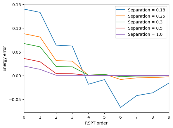
../../_images/d0f5446b23f6db3f74871813fa1549f03b5e491592aa0a15c1e769760cd3b7b7.png

As clearly seen, the convergence rate and even success depends critically on the state energy separation. This is due to the fact the a smaller energy separation leads to larger inverse matrix in the RSPT equation from which we determine the state vector correction $| Ψ^{(m)} ⟩$ .

Size extensivity in RSPT#

A system composed of two noninteracting subsystems has a Hamiltonian that is separable

\hat{H} = {\hat{H}}_{A} \otimes {\hat{I}}_{B} + {\hat{I}}_{A} \otimes {\hat{H}}_{B} \equiv {\hat{H}}_{A} + {\hat{H}}_{B}

where, in the last step, identity operators are left out and implicitly understood.

Zeroth- and first-order energies#

We assume that the unperturbed Hamiltonian (and thereby also the perturbation) is chosen as to also be separable. The zeroth-order wave function becomes

| Ψ_{A B}^{(0)} ⟩ = | Ψ_{A}^{(0)} ⟩ \otimes | Ψ_{B}^{(0)} ⟩

and the associated zeroth-order energy reads

E_{A B}^{(0)} = E_{A}^{(0)} + E_{B}^{(0)}

For the first-order energy correction, we straightforwardly get

E_{A B}^{(1)} = ⟨ Ψ_{A B}^{(0)} | \hat{V} | Ψ_{A B}^{(0)} ⟩ = E_{A}^{(1)} + E_{B}^{(1)}

Second-order energy#

The first-order wave function becomes

| Ψ_{A B}^{(1)} ⟩ = - ({\hat{H}}_{0} - E_{A B}^{(0)})^{- 1} (\hat{V} - E_{A B}^{(1)}) | Ψ_{A B}^{(0)} ⟩

Operators and energies within parenthesis are separable but we need to investigate the effect of the inverse operation.

Let us introduce ${\hat{Ω}}_{A} = {\hat{H}}_{0; A} - E_{A}^{(0)}$ and use the identity

- ({\hat{Ω}}_{A} + {\hat{Ω}}_{B})^{- 1} = - {\hat{Ω}}_{A}^{- 1} + ({\hat{Ω}}_{A} + {\hat{Ω}}_{B})^{- 1} {\hat{Ω}}_{B} {\hat{Ω}}_{A}^{- 1}

For the first of these two terms, we get

- {\hat{Ω}}_{A}^{- 1} ({\hat{V}}_{A} - E_{A}^{(1)}) | Ψ_{A}^{(0)} ⟩ = | Ψ_{A}^{(1)} ⟩

whereas for the second, we get

{\hat{Ω}}_{B} {\hat{Ω}}_{A}^{- 1} ({\hat{V}}_{A} - E_{A}^{(1)}) | Ψ_{A}^{(0)} ⟩ \otimes | Ψ_{B}^{(0)} ⟩ = 0

since

{\hat{Ω}}_{B} | Ψ_{B}^{(0)} ⟩ = 0

Collecting results for the two subsystems, the first-order correction to the wave function becomes

| Ψ_{A B}^{(1)} ⟩ = | Ψ_{A}^{(1)} ⟩ \otimes | Ψ_{B}^{(0)} ⟩ + | Ψ_{A}^{(0)} ⟩ \otimes | Ψ_{B}^{(1)} ⟩

and the second-order correction to the energy is thereby shown to fulfill

E_{A B}^{(2)} = ⟨ Ψ_{A B}^{(0)} | \hat{V} | Ψ_{A B}^{(1)} ⟩ = E_{A}^{(2)} + E_{B}^{(2)}

In other words, RSPT has been shown to be size-extensive up to second order in perturbation theory.