Core-valence separation#
The calculation of X-ray absorption spectra poses some additional problems, since the core-excited states are embedded in the continuum of valence-ionized states. This means that the targeted core-excited states cannot easily be resolved with, e.g., a Davidson approach, as a large number of valence-excited and -ionized states need to be converged first. In order to alleviate this issue, the core-valence separation (CVS) approach has been developed. The CVS approximation is based on the assumption that the core-excited and valence-excited states are coupled weakly, such that this coupling can be neglected. This approximation can be rationalized based on the large energetic and spatial separation between core- and valence-excited states. Indeed, as we will see in the following, the error introduced by the CVS approximation turns out to be very small. Neglecting the core-valence coupling blocks, the dimensionality of the pseudo-eigenvalue equation is greatly reduced, where the lowest energy eigenstates are now core-excitations:
with matrix blocks
with \(I\) and \(J\) restricted to the core orbitals.
As a test, we calculate the X-ray absorption spectrum of water, considering the full and reduce RPA.
Show code cell source
import copy
import adcc
import matplotlib.pyplot as plt
import numpy as np
import veloxchem as vlx

def lorentzian(x, y, xmin, xmax, xstep, gamma):
    xi = np.arange(xmin, xmax, xstep)
    yi = np.zeros(len(xi))
    for i in range(len(xi)):
        for k in range(len(x)):
            yi[i] = yi[i] + y[k] * (gamma / 2.0) / (
                (xi[i] - x[k]) ** 2 + (gamma / 2.0) ** 2
            )
    return xi, yi

au2ev = 27.211386
water_mol_str = """
O       0.0000000000     0.0000000000     0.1178336003
H      -0.7595754146    -0.0000000000    -0.4713344012
H       0.7595754146     0.0000000000    -0.4713344012
"""

basis = "6-31G"
vlx_mol = vlx.Molecule.read_molecule_string(water_mol_str)
vlx_bas = vlx.MolecularBasis.read(vlx_mol, basis)

scf_drv = vlx.ScfRestrictedDriver()
scf_settings = {"conv_thresh": 1.0e-6}
method_settings = {"xcfun": "b3lyp"}
scf_drv.update_settings(scf_settings, method_settings)
scf_results = scf_drv.compute(vlx_mol, vlx_bas)
Full-space results#
For the full-space results, we construct the Hessian and property gradients:
lr_eig_solver = vlx.LinearResponseEigenSolver()
lr_eig_solver.update_settings(scf_settings, method_settings)

lr_solver = vlx.LinearResponseSolver()
lr_solver.update_settings(scf_settings, method_settings)

# Electronic Hessian
E2 = lr_eig_solver.get_e2(vlx_mol, vlx_bas, scf_results)

# Property gradients for dipole operator
V1_x, V1_y, V1_z = lr_solver.get_prop_grad("electric dipole", "xyz", vlx_mol, vlx_bas, scf_results)

# Dimension
c = int(len(E2) / 2)

# Overlap matrix
S2 = np.identity(2 * c)
S2[c : 2 * c, c : 2 * c] *= -1
Calculating the excitation energies and oscillator strengths:
# Set up and solve eigenvalue problem
Sinv = np.linalg.inv(S2)  # for clarity - is identical
M = np.matmul(Sinv, E2)
eigs, X = np.linalg.eig(M)

# Reorder results
idx = np.argsort(eigs)
eigs = np.array(eigs)[idx]
X = np.array(X)[:, idx]

# Compute oscillator strengths
fosc = []
for i in range(int(len(eigs) / 2)):
    j = i + int(len(eigs) / 2)  # focus on excitations
    Xf = X[:, j]
    Xf = Xf / np.sqrt(np.matmul(Xf.T, np.matmul(S2, Xf)))
    tm = np.dot(Xf, V1_x) ** 2 + np.dot(Xf, V1_y) ** 2 + np.dot(Xf, V1_z) ** 2
    fosc.append(tm * 2.0 / 3.0 * eigs[j])
CVS-space results#
The dimensions of the CVS-space:
# Number of virtuals
nocc = vlx_mol.number_of_alpha_electrons()
nvirt = vlx_bas.get_dimensions_of_basis() - nocc
n = nocc * nvirt

# CVS space
res_mo = 1
res_indx = 0
c = res_mo * nvirt
Hessian and property gradients:
# Define starting index for deexcitation
c_int_deex = n + res_indx

# CVS Hessian
E2_cvs = np.zeros((2 * c, 2 * c))
E2_cvs[0:c, 0:c] = E2[res_indx:c, res_indx:c]
E2_cvs[0:c, c : 2 * c] = E2[res_indx:c, c_int_deex : c_int_deex + c]
E2_cvs[c : 2 * c, 0:c] = E2[c_int_deex : c_int_deex + c, res_indx:c]
E2_cvs[c : 2 * c, c : 2 * c] = E2[
    c_int_deex : c_int_deex + c, c_int_deex : c_int_deex + c
]

# CVS overlap matrix
S2_cvs = np.identity(2 * c)
S2_cvs[c : 2 * c, c : 2 * c] *= -1

# CVS property gradients
V1_cvs_x = np.zeros(2 * c)
V1_cvs_x[0:c] = V1_x[res_indx:c]
V1_cvs_x[c : 2 * c] = V1_x[c_int_deex : c_int_deex + c]
V1_cvs_y = np.zeros(2 * c)
V1_cvs_y[0:c] = V1_y[res_indx:c]
V1_cvs_y[c : 2 * c] = V1_y[c_int_deex : c_int_deex + c]
V1_cvs_z = np.zeros(2 * c)
V1_cvs_z[0:c] = V1_z[res_indx:c]
V1_cvs_z[c : 2 * c] = V1_z[c_int_deex : c_int_deex + c]
Calculating energies and intensities:
# Set up and solve eigenvalue problem
Sinv = np.linalg.inv(S2_cvs)  # for clarity - is identical
M = np.matmul(Sinv, E2_cvs)
eigs_cvs, X_cvs = np.linalg.eig(M)

# Reorder results
idx = np.argsort(eigs_cvs)
eigs_cvs = np.array(eigs_cvs)[idx]
X_cvs = np.array(X_cvs)[:, idx]

# Compute oscillator strengths
fosc_cvs = []
for i in range(int(len(eigs_cvs) / 2)):
    j = i + int(len(eigs_cvs) / 2)  # focus on excitations
    Xf_cvs = X_cvs[:, j]
    Xf_cvs = Xf_cvs / np.sqrt(np.matmul(Xf_cvs.T, np.matmul(S2_cvs, Xf_cvs)))
    tm_cvs = (
        np.dot(Xf_cvs, V1_cvs_x) ** 2
        + np.dot(Xf_cvs, V1_cvs_y) ** 2
        + np.dot(Xf_cvs, V1_cvs_z) ** 2
    )
    fosc_cvs.append(tm_cvs * 2.0 / 3.0 * eigs_cvs[j])
From VeloxChem#
The CVS-space approach is implemented in VeloxChem and can be done by the LinearResponseEigenSolver class. To run CVS calculation, set core_excitation to True and num_core_orbitals to the number of core orbitals to be included.
In this example we only need to include one core orbital (O1s in water molecule).
lr_eig_solver.core_excitation = True
lr_eig_solver.num_core_orbitals = 1
lr_eig_solver.nstates = 3
vlx_cvs_results = lr_eig_solver.compute(vlx_mol, vlx_bas, scf_results)
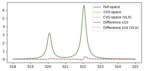
Comparison#
Comparing the obtained spectra:
plt.figure(figsize=(6,3))

x, y = eigs[int(len(eigs) / 2) :], fosc
x1, y1 = lorentzian(x, y, 518 / au2ev, 525 / au2ev, 0.001, 0.3 / au2ev)
plt.plot(x1 * au2ev, y1)

x, y = eigs_cvs[int(len(eigs_cvs) / 2) :], fosc_cvs
x2, y2 = lorentzian(x, y, 518 / au2ev, 525 / au2ev, 0.001, 0.3 / au2ev)
plt.plot(x2 * au2ev, y2, linestyle='--')

x, y = vlx_cvs_results['eigenvalues'], vlx_cvs_results['oscillator_strengths']
x3, y3 = lorentzian(x, y, 518 / au2ev, 525 / au2ev, 0.001, 0.3 / au2ev)
plt.plot(x3 * au2ev, y3, linestyle=':')

plt.plot(x1 * au2ev, 10*(y1 - y2), linestyle='--')
plt.plot(x1 * au2ev, 10*(y1 - y3), linestyle=':')

plt.legend(("Full-space", "CVS-space", "CVS-space (VLX)", "Difference x10", "Difference x10 (VLX)"))
plt.tight_layout()
plt.show()
Or considering the results for the full set of eigenstates:
plt.figure(figsize=(6,3))
plt.bar(27.2114*eigs[int(len(eigs) / 2) :], fosc, width=4.0)
plt.bar(27.2114*eigs_cvs[int(len(eigs_cvs) / 2) :], fosc_cvs, width=4.0)
plt.plot(27.2114*eigs[int(len(eigs) / 2) :], fosc, 'x')

plt.tight_layout()
plt.show()
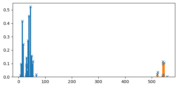
Where we see that, as expected, the full-space results have many states at lower energies, but essentially the same at high (core-excitation) energies.