Choice of coordinates

A fundamental concept in quantum chemistry is the multi-dimensional potential energy surface (PES). It captures the interplay between the electronic and nuclear degrees of freedom in a system, and stationary points on the PES are important in elucidating molecular conformations and explaining the mechanisms of chemical and photo-chemical reactions. The first- (gradient) and second-order (Hessian) derivatives of the energy with respect to nuclear displacements are key elements in locating these points (minima and transition states) and determining minimum energy reaction pathways.

We will here discuss the choice of coordinates in which these energy derivatives are expressed.

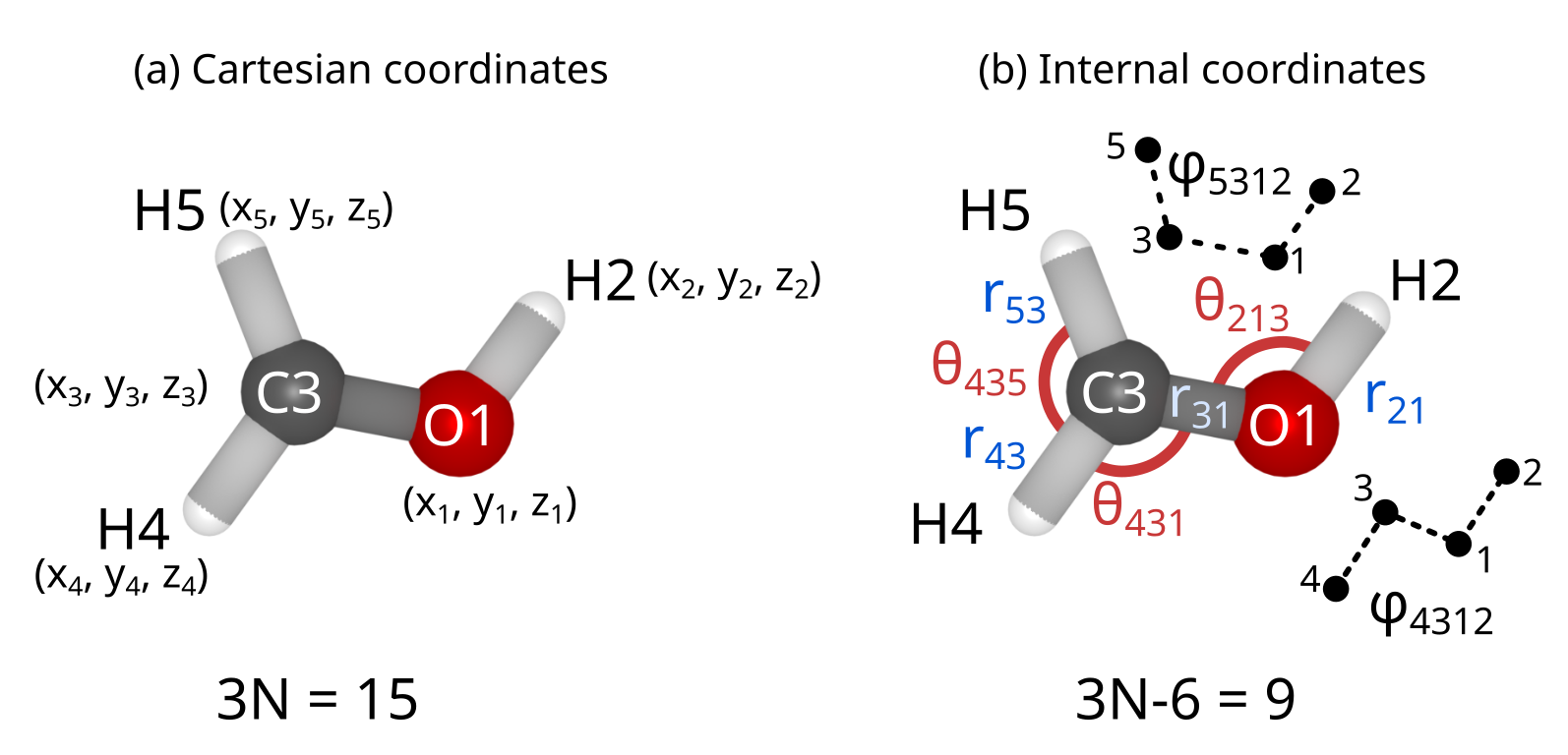
Cartesian coordinates

The most straightforward way to define atomic positions is to use a Cartesian reference system and define each atomic position in terms of its \((x,y,z)\)-coordinates. In this coordinate system it is very easy to determine the total energy and energy gradient, but this choice is not favorable for geometry optimization because these coordinates are strongly coupled to one another.

Internal coordinates

A more favorable choice is to work with internal coordinates, such as bond lengths, valence angles and dihedrals. The most well known set of internal coordinates is the Z-matrix, which uses this properties in order to describe the molecular structure. However, using internal coordinates poses two challenges: (1) the choice of coordinates is not unique, and (2) internal coordinates have to be transformed back into Cartesian coordinates to compute the energy and gradient. Several ways of handling these problems are discussed below.

Transforming between coordinate systems

Given the set of internal coordinates \(\mathbf{q}=(q_1,q_2,...,q_{n_q})\), we would like to relate displacements performed in these coordinates to displacements in the \(n_x=3N\) Cartesian coordinates \(\mathbf{x}=(x_1,x_2,...,x_{n_x})\) (to simplify, we denoted all Cartesian coordinates by \(x\)). For this purpose, we define matrix \(\mathbf{B}\) (called the Wilson \(\mathbf{B}\)-matrix) [Neal09]

\[ B_{ij} = \frac{\partial q_i}{\partial x_j} \]

To determine the changes in \(\mathbf{x}\) as a result of changes performed in \(\mathbf{q}\), we basically need to obtain the inverse relation \(\partial x_j/\partial q_i\). However, because \(\mathbf{B}\) is generally rectangular and cannot be directly inverted, we first have to construct a square matrix \(\mathbf{G}\)

\[ \mathbf{G} = \mathbf{B}\mathbf{B}^\mathrm{T} \]

If we are using non-redundant internal coordinates, \(\mathbf{G}\) can be inverted directly. However, if the internal coordinates are redundant, some of the rows of \(\mathbf{G}\) will be linearly dependent. In this case, we have to set up and solve an eigenvalue equation that will allow us to separate out the redundancies [PF92]

\[\begin{split} \mathbf{G} \begin{pmatrix} \mathbf{U} & \mathbf{R} \end{pmatrix} = \begin{pmatrix} \mathbf{U} & \mathbf{R} \end{pmatrix} \begin{bmatrix} \boldsymbol{\Lambda} & 0 \\ 0 & 0 \end{bmatrix} \end{split}\]

This equation has \(n=3N-6\) (or \(3N-5\) for linear molecules) non-zero eigenvalues and \(n_q-n\) zero eigenvalues. The non-zero eigenvalues correspond to linearly independent coordinates, while those which are zero identify the redundant ones. Furthermore, the first \(n\) eigenvectors contained in the matrix \(\mathbf{U}\) are non-redundant and can be used to define a set of non-redundant coordinates \(\mathbf{s}\):

\[ \mathbf{s} = \mathbf{U}^\mathrm{T} \mathbf{q} \]

The eigenvalue equation can be used to define a generalized inverse matrix \(\mathbf{G}^{-}\):

\[\begin{split} \mathbf{G}^{-} = \begin{pmatrix} \mathbf{U} & \mathbf{R} \end{pmatrix} \begin{bmatrix} \boldsymbol{\Lambda}^{-1} & 0 \\ 0\,\,\,\,\,\,\,\, & 0 \end{bmatrix} \begin{pmatrix} \mathbf{U}^\mathrm{T}\\ \mathbf{R}^\mathrm{T} \end{pmatrix} \end{split}\]

which, in turn, is used to determine the transformation between Cartesian and internal coordinates displacements [WS16]:

\[ \Delta\mathbf{x} = \mathbf{B}^\mathrm{T}\mathbf{G}^{-}\Delta\mathbf{q} \]

In a similar way, the gradient can be transformed from Cartesian to internal coordinates [Neal09]:

\[ \mathbf{g}_q = \mathbf{G}^{-}\mathbf{B}\mathbf{g}_x \]

where we have denoted the gradient in Cartesian coordinates by \(\mathbf{g}_x\) and the gradient in internal coordinates by \(\mathbf{g}_q\).

With these equations we can now transform a displacement in internal coordinates to a displacement in Cartesian coordinates, compute the energy gradient, and transform the gradient back to internal coordinates.

In the case of the Hessian matrix, the transformation to internal coordinates requires the second-order derivatives of \(q_i\) with respect to the Cartesian coordinates \(x_j\), \(x_k\)

\[ B^{(2)}_{ijk} = \frac{\partial^2 q_i}{\partial x_j\partial x_k} \]

These derivatives, together with \(\mathbf{G}^{-}\), the Wilson \(\mathbf{B}\)-matrix and gradient are then used to transform the Hessian from Cartesian (\(\mathbf{H}_x\)) to internal (\(\mathbf{H}_q\)) coordinates

\[ \mathbf{H}_q = \mathbf{G}^{-} \mathbf{B} \left[ \mathbf{H}_x - \mathbf{g}_q \mathbf{B}^{(2)}\right]\mathbf{B}^\mathrm{T} \mathbf{G}^{-\mathrm{T}} \]

After these transformations are carried out, further transformations to related internal coordinates, for example to use \(1/R\) instead of \(R\) (bond length), are easy to implement, as exemplified for the gradient: Given the gradient in terms of \(R\)

\[ g(R) = \frac{\mathrm{d} E}{\mathrm{d}R} \]

the transformation to \(u=1/R\) is a simple change of variables

\[ g(u) = \frac{\mathrm{d} E}{\mathrm{d}u}=\frac{\mathrm{d} E}{\mathrm{d}R}\frac{\mathrm{d} R}{\mathrm{d}u} = \frac{\mathrm{d} E}{\mathrm{d}R}\frac{\mathrm{d} u^{-1}}{\mathrm{d}u} = -u^{-2}\,g(R) = -R^{2} \,g(R) \]

The transformation of the Hessian can be carried out similarly.