MCSCF#
Strong/static correlation#
As we can see from perturbation theory, the largest contributions to the correlation energy typically comes from small denominators, that is from excitations from and to orbitals around the Fermi level. This suggest using a multi-scale approach to correlation, with an accurate method to describe correlation coming from a few orbitals located near the Fermi level and a cheaper but less accurate method for the rest.
In particular, in some situations, a few orbitals can have such large correlation effects that most electronic structure methods fail, sometimes dramatically. In those situations, the Hartree-Fock reference, upon which most other electronic structure methods are based, is not even qualitatively correct. One of the few methods able to describe such systems is configuration interaction, which then shows several determinants with significant weights.
One simple example of this is what happens during homolytic bond dissociation.
import veloxchem as vlx
import multipsi as mtp
import numpy as np
import matplotlib.pyplot as plt
import scipy.linalg
# HF and CI calculation of OH.

mol_str="""
O 0.0000 0.0000  0.0000
H 0.0000 0.8957 -0.3167
"""
molecule = vlx.Molecule.read_molecule_string(mol_str, units='angstrom')
molecule.set_multiplicity(2)
basis = vlx.MolecularBasis.read(molecule, "STO-3G", ostream=None)
scf_drv = vlx.ScfUnrestrictedDriver()
scf_drv.ostream.mute()
scf_results = scf_drv.compute(molecule, basis)
E_OH_hf = scf_drv.get_scf_energy()

space = mtp.OrbSpace(molecule,scf_drv.mol_orbs)
space.fci()
CIdrv = mtp.CIDriver()
ci_results = CIdrv.compute(molecule, basis, space)
E_OH_FCI = ci_results["energies"][0]

# HF calculation of H, equivalent to CI

mol_str = "H 0.0000 0.0000 0.0000"
molecule = vlx.Molecule.read_molecule_string(mol_str, units='angstrom')
molecule.set_multiplicity(2)
basis = vlx.MolecularBasis.read(molecule, "STO-3G", ostream=None)
scf_results = scf_drv.compute(molecule, basis)
E_H_hf = scf_drv.get_scf_energy()

# HF and CI calculations of water with stretching of one O-H bond

mol_template = """
O 0.0000 0.0000  0.0000
H 0.0000 0.8957 -0.3167
H 0.0000 0.0000  OHdist
"""
scf_drv = vlx.ScfRestrictedDriver()
scf_drv.ostream.mute()
scf_drv.max_iter = 200

distlist = []
E_hf = []
E_FCI = []
NON = []

# Scan over O-H distances
for dist in [0.7,0.8,0.9,0.95,1.1,1.3,1.5,1.7,2,2.5,3,3.5,4,4.5,5]:
    mol_str = mol_template.replace("OHdist", str(dist))
    molecule = vlx.Molecule.read_molecule_string(mol_str, units='angstrom')
    basis = vlx.MolecularBasis.read(molecule, "STO-3G", ostream=None)
    scf_results = scf_drv.compute(molecule, basis)
    if scf_drv.is_converged:
        distlist.append(dist)
        E_hf.append(scf_drv.get_scf_energy() - E_H_hf - E_OH_hf)

        space=mtp.OrbSpace(molecule,scf_drv.mol_orbs)
        space.fci()
        ci_results = CIdrv.compute(molecule,basis,space)
        E_FCI.append(ci_results["energies"][0] - E_H_hf - E_OH_FCI)
        NON.append(ci_results["natural_occupations"][0]) # Get the natural occupation numbers
plt.figure(figsize=(6,4))
plt.title('Energy during O-H dissociation')
x = np.array(distlist)
y = np.array(E_FCI)
z = np.array(E_hf)
plt.plot(x,y, label='FullCI')
plt.plot(x,z, label='RHF')
plt.legend()
plt.tight_layout(); plt.show()
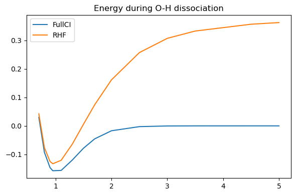
It is clear that while HF gives a reasonable energy around the equilibrium, it performs very poorly at longer O-H distances, failing to reach the sum of the energies of the two fragments OH\(^.\) and H\(^.\)). The SCF convergence is also very poor and can in some cases even fail.
The explanation can be found by looking at the occupation numbers of the CI, which shows that two orbitals are getting increasingly correlated. If we would plot them, we would see they correspond to the \(\sigma\) and \(\sigma^*\) orbitals.
Note
The natural orbitals are sorted by occupation numbers, so the most correlated are the “highest” of the HF occupied and the “lowest” of the HF empty.
plt.figure(figsize=(6,4))
plt.title('Natural occupation numbers during O-H dissociation')
x = np.array(distlist)
sigma=[]
sigma_star=[]
for NONi in NON:
    sigma.append(NONi[4])
    sigma_star.append(NONi[5])
y = np.array(sigma)
z = np.array(sigma_star)
plt.plot(x, y, label='sigma')
plt.plot(x, z, label='sigma*')
plt.legend()
plt.tight_layout(); plt.show()
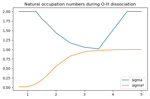
Clearly, at longer distances, the Hartree-Fock approximation of doubly occupied \(\sigma\) and empty \(\sigma^*\) becomes less and less reasonable.
On the other hand, even at long O-H distances, all occupation numbers remain reasonably close to the HF assumption, suggesting that we only needed to perform the CI over these two orbitals.
print("Natural orbital occupation numbers at 5 Å")
print(NON[-1])
Natural orbital occupation numbers at 5 Å
[1.9999994  1.9986901  1.97454437 0.9998077  1.99931509 1.0001923
 0.02745103]
Doing so would define an “active space” containing the two orbitals, while the other orbitals would be called “inactive”. Including all excitations within this active space, that performing a full CI within this small space, we define a so-called “complete active space” (CAS), and the method is thus called CASCI.
The Multiconfigurational Self-Consistent Field method (MCSCF)#
While the CASCI can be performed after a Hartree-Fock calculation, it has a major flaw in that the orbitals were optimized assuming the Hartree-Fock density was reasonable. But the main motivation behind CASCI was precisely that the Hartree-Fock density was wrong, and thus the Hartree-Fock orbitals are far from optimal. It is thus tempting to want to optimize the orbitals using the CASCI density. Of course, as the orbitals change, it is likely the CASCI would also need to be relaxed. Clearly, the process need to be self-consistent. The resulting method is called the multiconfigurational self-consistent field method (MCSCF), and if we used a complete active space, it can be called more specifically CASSCF.
MCSCF can be seen as a generalization of the self-consistent field concept of Hartree-Fock to a wavefunction containing several determinants. It simultaneously relaxes the orbitals and the CI coefficients.
Illustrative example#
Let us illustrate the MCSCF method by applying it to our O-H dissociation problem. As we mentioned, an active space containing the \(\sigma\) and \(\sigma^*\) is enough to qualitatively describe the bond-breaking. The simplest way to define this active space in the program is to mention the number of active orbitals (here 2) as well as the number of electrons in them (here also 2). We often use the notation CAS(\(m,n\)) with \(m\) the number of electrons and \(n\) the number of orbitals.
E_CASSCF=[]

Mcscf_drv=mtp.McscfDriver()

#Scan over O-H distances
for dist in distlist:
    mol_str = mol_template.replace("OHdist", str(dist))
    molecule = vlx.Molecule.read_molecule_string(mol_str, units='angstrom')
    basis = vlx.MolecularBasis.read(molecule, "STO-3G")
    scf_results = scf_drv.compute(molecule, basis)

    space = mtp.OrbSpace(molecule, scf_drv.mol_orbs)
    space.cas(2,2)
    mcscf_results = Mcscf_drv.compute(molecule, basis, space)
    E_CASSCF.append(mcscf_results["energies"][0] - E_H_hf - E_OH_hf)
plt.figure(figsize=(6,4))
plt.title('Energy during O-H dissociation')
x = np.array(distlist)
y = np.array(E_FCI)
z = np.array(E_hf)
zz = np.array(E_CASSCF)
plt.plot(x,y, label='FullCI')
plt.plot(x,z, label='RHF')
plt.plot(x,zz, label='CASSCF')
plt.legend()
plt.tight_layout(); plt.show()
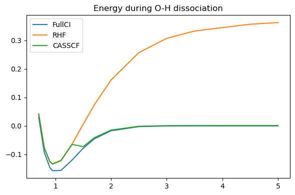
The result looks a bit disappointing. On one side, the MCSCF converges without major issue (unlike Hartree-Fock) and indeed approaches the FCI result at long distances. However, at short distances it did no better than HF, resulting in a weird transition between the two zones.
To understand why, let’s visualize the Hartree-Fock orbitals for a distance of 1.1 Å.
# Run again the 1.1 Å Hartree-Fock
mol_str = mol_template.replace("OHdist", "1.1")
molecule = vlx.Molecule.read_molecule_string(mol_str, units='angstrom')
basis = vlx.MolecularBasis.read(molecule, "STO-3G")
scf_results = scf_drv.compute(molecule, basis)
viewer = mtp.OrbitalViewer()
viewer.plot(molecule, basis, scf_drv.mol_orbs)
This highlights one of the main difficulties in MCSCF. It is not enough to provide the number of active orbitals, it is essential to provide the right ones. By default, our CAS(2,2) includes the HOMO and LUMO of our starting HF orbitals, but at 1.1 Å, the HOMO is an oxygen lone pair, not the \(\sigma\). We can fix this by explicitely requesting the HOMO-1 in this case.
We could visualize the starting orbitals for every geometry, but an easier alternative is to visualize a single structure, and then use these orbitals and active space as a starting point for all the other structures. The hope is that the active space will be stable over the entire scan (similarly for optimization or dynamics).
Generally, the stronger the correlation, the more stable is the active space. Thus, here, the best strategy is to start from the long distances and then scan backwards.
E_CASSCF=[]

# Initialise our first guess to 2 Å
mol_str = mol_template.replace("OHdist", "2")
molecule = vlx.Molecule.read_molecule_string(mol_str, units='angstrom')
basis = vlx.MolecularBasis.read(molecule, "STO-3G")
scf_results = scf_drv.compute(molecule, basis)

space = mtp.OrbSpace(molecule, scf_drv.mol_orbs)
space.cas(2,2)

# Scan over O-H distances in reverse order
for dist in distlist[::-1]:
    mol_str = mol_template.replace("OHdist", str(dist))
    molecule = vlx.Molecule.read_molecule_string(mol_str, units='angstrom')

    mcscf_results = Mcscf_drv.compute(molecule, basis, space)
    E_CASSCF.append(mcscf_results["energies"][0] - E_H_hf - E_OH_hf)

E_CASSCF = E_CASSCF[::-1] # Reorder the energies
plt.figure(figsize=(6,4))
plt.title('Energy during O-H dissociation')
x = np.array(distlist)
y = np.array(E_FCI)
z = np.array(E_hf)
zz = np.array(E_CASSCF)
plt.plot(x, y, label='FullCI')
plt.plot(x, z, label='RHF')
plt.plot(x, zz, label='CASSCF')
plt.legend()
plt.tight_layout(); plt.show()
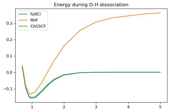
We now have a smooth curve that is nearly as good (in this minimal basis case where correlation outside of the active space is limited) as the full CI.
Overall, it is always a good idea to check the starting orbitals you provide, as well as the final orbitals (after convergence).
Theory#
In order to understand the theory below, it is recommended to first read the chapter on Hartree-Fock and Configuration Interaction as this section borrows extensively from both.
The MCSCF wavefunction contains both CI and orbital parameters and can be written as
with \(\hat{\kappa}\) the orbital rotation operator
It is often simpler to treat the optimization as two separate problems, an optimization of the CI coefficients followed by an optimization of the orbitals. Doing so means neglecting the coupling between the two occuring in the Hessian (\(\frac{\partial^2 E}{\partial c_I \partial \kappa_{pq}}\)), and the method is thus “first order”.
The CI optimization can be done following the standard CI techniques seen in a previous chapter. However, the orbital optimization needs more inspection. The general expression of the orbital derivative is
with
with \(\mathbf{D}\) and \(\boldsymbol{\Gamma}\) being the one and two-particle density matrices, respectively. For a Hartree-Fock wavefunction, the one-particle density is diagonal with an occupation number of 2 for all occupied orbitals and \(\Gamma_{pqrs} = D_{pq}D_{rs} - \frac{1}{2} D_{pr}D_{qs}\) , and the equation then simplifies to the usual Fock matrix
The MCSCF matrix is more complicated, and we can see two cases depending on if \(p\) is inactive or active
and
where we have used the indices \(i, j\) for inactive orbitals, \(t,u, v, w\) for active and \(a,b\) for virtual. The matrices \(D_{tu}\) and \(\Gamma_{tuvw}\) are the active one and two-particle density matrices computed by the CI code.
By defining the inactive Fock matrix \(F^\mathrm{I}_{pq} = h_{pq} + \sum_j 2(pq|jj) - (pj|qj)\), we can simplify these expressions somewhat
and
Since this matrix is analogous to the HF Fock matrix, it is usually called the effective Fock matrix.
In HF, the Fock matrix is diagonalized, and it is easy to see how doing so indeed sets the gradient \(2(F_{pq}-F_{qp})\) to 0. However, the MCSCF matrix is not symmetric and cannot in general be diagonalized. Note that the inactive-inactive block looks very similar to a Hartree-Fock Fock matrix and can be diagonalized, which defines the orbital energies for the inactive orbitals.
Since we cannot diagonalize the MCSCF Fock matrix, we need to find a different way to set the gradient to 0. Different techniques exist, but one of the most popular is to use the Newton method.
The Newton method is a second order method, which means it makes use of the second derivatives to improve the rate of convergence. According to this method, the optimal displacement \(\mathbf{X}\) to fulfill convergence is given by
with the Hessian \(\mathbf{H}\) and gradient \(\mathbf{G}\).
However, even approximate second derivatives can lead to fast convergence of the method, and as mentioned above, here we will neglect the coupling between CI and orbital parameters that occur in a full Newton algorithm. Similarly, the exact orbital-orbital Hessian includes integrals in the molecular orbital (MO) basis with inactive and virtual indices. Since the transformation to the MO basis is expensive, we want to restrict it to only active indices (which are needed for the CI). It is thus customary to use an approximation even for the orbital-orbital Hessian which uses only matrix elements already used for the gradients and is diagonal:
Implementation#
With all the equations set up, we can now implement a MCSCF. We are going to make use of the CI module in MultiPsi (a CI implementation is suggested in a previous section) as well as the integrals modules of Veloxchem.
Let’s consider a moderately stretched water molecule with starting orbitals computed at the HF level.
water_stretched = """
O 0.0000 0.0000  0.0000
H 0.0000 0.8957 -0.3167
H 0.0000 0.0000  1.5
"""
molecule = vlx.Molecule.read_molecule_string(water_stretched, units='angstrom')
scf_drv = vlx.ScfRestrictedDriver()
scf_drv.ostream.mute()
scf_results = scf_drv.compute(molecule, basis)
We can reuse the code we wrote in the Configuration Interaction section to compute the inactive Fock matrix, energy and the active 2-electron integrals:
nbas = basis.get_dimensions_of_basis()

V_nuc = molecule.nuclear_repulsion_energy()

# one-electron Hamiltonian
kinetic_drv = vlx.KineticEnergyDriver()
T = kinetic_drv.compute(molecule, basis).full_matrix().to_numpy()

nucpot_drv = vlx.NuclearPotentialDriver()
V = -nucpot_drv.compute(molecule, basis).full_matrix().to_numpy()

h = T + V

# two-electron Hamiltonian
fock_drv = vlx.FockDriver()
g = fock_drv.compute_eri(molecule, basis)

def CI_integrals(C, nIn, nAct, h,g):
    Cact = C[:, nIn:nIn+nAct] # Active MOs

    # Compute the inactive Fock matrix
    Din = np.einsum('ik,jk->ij', C[:, :nIn], C[:, :nIn]) #inactive density
    Jin = np.einsum('ijkl,kl->ij', g, Din)
    Kin = np.einsum('ilkj,kl->ij', g, Din)
    Fin = h + 2*Jin - Kin

    # Transform to MO basis
    Ftu = np.einsum("pq, qu, pt->tu", Fin, Cact, Cact)

    # Inactive energy:
    Ein = np.einsum('ij,ij->', h + Fin, Din) + V_nuc

    # Compute the MO 2-electron integrals
    pqrw = np.einsum("pqrs,sw->pqrw", g   , Cact)
    pqvw = np.einsum("pqrw,rv->pqvw", pqrw, Cact)
    puvw = np.einsum("pqvw,qu->puvw", pqvw, Cact)
    # Above intermediate will also be used later
    tuvw = np.einsum("puvw,pt->tuvw", puvw, Cact)
    return Ein, Ftu, tuvw, Fin, puvw
Using this, we can implement the MCSCF iterations:
max_iter = 40
conv_thresh = 1e-4

space=mtp.OrbSpace(molecule, scf_drv.mol_orbs) # MolSpace will store the orbitals for us
space.cas(2,2)

nIn = space.n_inactive # Number of inactive orbitals
nAct = space.n_active # Number of active orbitals

CIdrv = mtp.CIDriver(ostream="silent") # Deactivate printing

print("iter    MCSCF energy    Error norm")

for iter in range(max_iter):
    C = space.molecular_orbitals.alpha_to_numpy()
    Cact = C[:, nIn:nIn+nAct] #Active MOs

    # Obtain the integrals needed for CI
    Ein, Ftu, tuvw, Fin, puvw = CI_integrals(C, nIn, nAct, h, g)

    # Feed them to the CI driver and compute the CI energy
    CIdrv._update_integrals(Ein, Ftu, tuvw)
    ci_results = CIdrv.compute(molecule, basis, space) #Compute only the ground state
    E = ci_results["energies"][0]

    # Obtain CI densities
    Dact = CIdrv.get_active_density(0)
    D2act = CIdrv.get_active_2body_density(0)

    # Active Fock matrix
    Dact_pq = np.einsum("tu,pt,qu->pq", Dact, Cact, Cact) #Transform to AO basis
    Jact = np.einsum('ijkl,kl->ij', g, Dact_pq)
    Kact = np.einsum('ilkj,kl->ij', g, Dact_pq)
    Fact = 2 * Jact - Kact

    # Form effective Fock matrix
    Feff = np.zeros((nbas,nbas))
    Feff[:nIn,:] = np.einsum("pq,pt,qn->tn", 2*Fin+Fact, C[:, :nIn], C) #Fiq
    Feff[nIn:nIn+nAct,:] = np.einsum("tu,pu,pq,qn->tn", Dact, Cact, Fin, C) #Ftq (1)
    Feff[nIn:nIn+nAct,:] += np.einsum("quvw,tuvw,qn->tn", puvw, D2act, C) #Ftq (2)

    # Form gradient 2(Fpq-Fqp)
    G = 2 * (Feff - np.transpose(Feff))

    # Check convergence
    e_vec = np.reshape(G, -1)
    error = np.linalg.norm(e_vec)
    print(f'{iter+1:>2d}  {E:16.8f}  {error:10.2e}')
    if error < conv_thresh:
        print('MCSCF iterations converged!')
        break

    # Extract some diagonals
    diag1 = np.einsum("pq,pm,qm->m", 2*Fin+Fact, C, C) # Diagonal of 2*Fin+Fact in MO basis
    diag2 = np.diagonal(Feff) # Diagonal of the effective Fock matrix

    # Form Hessian diagonal
    Hess = np.zeros((nbas,nbas))
    Hess[:nIn,nIn:] = 2* diag1[nIn:] - 2* diag1[:nIn].reshape(-1,1) #Sum of a line and column vectors
    Hess[nIn:nIn+nAct,:] = - 2 * diag2[nIn:nIn+nAct].reshape(-1, 1)
    Hess[nIn:nIn+nAct,nIn+nAct:] += np.einsum('tt,a->ta',Dact,diag1[nIn+nAct:])
    Hess[nIn:nIn+nAct,:nIn] += np.einsum('tt,a->ta',Dact,diag1[:nIn])
    Hess += np.transpose(Hess)
    Hess[:nIn,:nIn] = 1 # To avoid division by 0
    Hess[nIn + nAct:, nIn + nAct:] = 1 # To avoid division by 0

    # Finally, compute next step
    X = G / Hess
    expX = scipy.linalg.expm(X)
    newmo = np.matmul(C,expX)

    ene = np.zeros(nbas)
    occ = np.zeros(nbas)
    newmolorb = vlx.MolecularOrbitals([newmo], [ene], [occ], vlx.molorb.rest)
    space.molecular_orbitals = newmolorb
iter    MCSCF energy    Error norm
 1      -74.88252747    2.25e-01
 2      -74.89753572    6.02e-02
 3      -74.89903251    2.29e-02
 4      -74.89930538    1.40e-02
 5      -74.89938498    9.82e-03
 6      -74.89941463    6.75e-03
 7      -74.89942666    4.54e-03
 8      -74.89943169    3.03e-03
 9      -74.89943383    2.01e-03
10      -74.89943474    1.33e-03
11      -74.89943514    8.84e-04
12      -74.89943531    5.86e-04
13      -74.89943538    3.89e-04
14      -74.89943542    2.58e-04
15      -74.89943543    1.71e-04
16      -74.89943544    1.14e-04
17      -74.89943544    7.55e-05
MCSCF iterations converged!
# Compare to the MCSCF driver of multipsi
space = mtp.OrbSpace(molecule, scf_drv.mol_orbs)
space.cas(2,2)

Mcscf_drv = mtp.McscfDriver()
mcscf_results = Mcscf_drv.compute(molecule, basis, space)
MultiPsi uses several tools to accelerate convergence, in particular a Hessian update to fix for the fact that we are using an approximate Hessian, but this is beyond the scope of this chapter.
Multireference correlation#
For any reasonable size molecule, the active space will be but a fraction of the total orbital space, and thus, MCSCF provides only a small (though important) fraction of the total correlation. We typically say, somewhat incorrectly, that MCSCF captures the static correlation but still lacks dynamical correlation.
However, the same way as MCSCF can be seen as an extension of Hartree-Fock to the multiconfigurational case, there exists extensions of standard correlation methods (MP2, truncated CI, coupled cluster and even DFT) to the multiconfigurational case. However, several complications arise when generalizing single reference correlation to the multiconfigurational case, and several multireference variants exist for each single reference correlation method.
One of the most important difficulty in wavefunction-based multireference correlation is the choice of the n-particle basis. Let’s look at CISD and its multireference (MR) equivalent MRCISD as an example, though the discussion is very similar for multireference perturbation theory and multireference coupled cluster.
In CISD, the correlated wavefunction is expanded on a basis of singly and doubly excited determinants. Those are generated by applying excitation operators to the reference (Hartree-Fock) wavefunction \(| 0 \rangle\) :
The number of such functions is \(N_\mathrm{O}^2 N_\mathrm{V}^2\) with \(N_\mathrm{O}\) and \(N_\mathrm{V}\) the number of occupied and virtual orbitals respectively. These functions form an orthonormal basis and are orthogonal to the reference function.
A MCSCF wavefunction is already a linear combination of Slater Determinant:
We thus have 2 ways to generate our MRCISD functions. The first is to apply the excitation operators to each \(| \mathbf{I} \rangle\) function:
Note that we only write the \(ijab\) excitation but the MRCISD basis also needs to include excitations to and from the active orbitals.
These \(| \Psi_{ijab\mathrm{I}} \rangle \) have the same desirable property of forming an orthonormal basis. However, there are many of them, on the order of \(N_\mathrm{O}^2 N_\mathrm{V}^2 N_{CI}\) with \(N_{CI}\) the (potentially very large) number of determinants in our MCSCF. Let’s see this number in the example of a water CAS(6,5):
h2o_xyz = """3
water
O    0.000000000000        0.000000000000        0.000000000000
H    0.000000000000        0.740848095288        0.582094932012
H    0.000000000000       -0.740848095288        0.582094932012
"""

molecule = vlx.Molecule.read_xyz_string(h2o_xyz)

basis = vlx.MolecularBasis.read(molecule, "6-31G")

scf_drv = vlx.ScfRestrictedDriver(ostream=vlx.OutputStream(None))
scf_results = scf_drv.compute(molecule, basis)

space = mtp.OrbSpace(molecule,scf_drv.mol_orbs)
space.cisd()

expansion = mtp.CIExpansion(space)

print("Number of CISD Determinants  :", expansion.n_determinants)

space.cas(6,5)

expansion = mtp.CIExpansion(space)
print("Number of MCSCF Determinants :", expansion.n_determinants)

space.mrcisd()

expansion = mtp.CIExpansion(space)

print("Number of MRCISD Determinants:", expansion.n_determinants)
Number of CISD Determinants  : 2241
Number of MCSCF Determinants : 100
Number of MRCISD Determinants: 62490
Even with this very small active space, the number of MRCISD determinants become significantly larger than a standard CISD.
Alternatively, we could write our MRCISD expansion in a similar way to the CISD, by applying the excitation operators directly to the entire MCSCF wavefunction
In Multireference theory, the excitations within the active space are called internal excitations, thus the formulation above where those excitations are fixed to the MCSCF converged result is called “internal contraction”.
The advantage of this formulation is rather obvious. The size of our basis is now on the order of that of a standard CISD (differing only by the inclusion of occupied to active and active to virtual excitations). However, those functions are now significantly harder to manipulate. Each function is not a Slater Determinant but a linear combination of them, and in particular, this means that those functions are not all orthonormal. To see this, let’s take the specific example of \(itua\) excitations, that is a double excitation with one electron excited from inactive to active and one from active to virtual. The overlap between 2 such excitations with the same \(i\) and \(a\) but different active orbitals is:
which is related to the active 2-body density matrix and is not in general 0.
These complications get even worse when computing Hamiltonian matrix elements between such determinants, and thus, straightforward implementation of MRCISD involves up to 5-particle density matrix in the active space.
Some tricks have been found to reduce this number, but those internally contracted methods remain definitely more complex to implement than the uncontracted ones. Also, the additional flexibility in uncontracted method makes them slightly more accurate. Still the superior performance of internally contracted methods when medium to large active spaces are used makes them very attractive for the user. Below is a summary of some of the main multireference methods in existence.
Single reference method |
Uncontracted MR method |
Internally contracted MR |
|---|---|---|
MP2 |
MRMP2 |
CASPT2, NEVPT2 |
CISD |
MRCISD |
ic-MRCISD |
CCSD |
Mk-MRCCSD |
ic-MRCCSD |
MultiPsi currently only implements an uncontracted MRCISD. The workflow is to first compute a MCSCF and then add a MRCISD on top of it:
space.cas(6,5)

mcscf_drv = mtp.McscfDriver()
mcscf_results = mcscf_drv.compute(molecule,basis,space)

space.mrcisd() # Assumes a CAS has been defined before
#cidrv = mtp.CIDriver()
#mrci_results = cidrv.compute(molecule,basis,space)
Note that a MCSCF wavefunction satisfies the extended Brillouin theorem, which is a generalization of the Brillouin theorem of Hartree-Fock saying that the MCSCF wavefunction does not interact with single excitations. Because of this, internally contracted MRCIS does not improve upon the ground state MCSCF energy, in the same way as CIS does not improve upon HF. However, uncontracted MRCIS does bring some correlation as it allows a single excitation outside the active space to correlate with internal excitations.
space.cas(6,5)
space.mrcis()

#cidrv = mtp.CIDriver()
#mrcis_results = cidrv.compute(molecule,basis,space)
#print("Uncontracted MRCIS dynamical correlation:",
#          mrcis_results["energies"][0]-mcscf_results["energies"][0])