Absorption#
This section currently focus on the calculation of absorption spectra, with vibrational effects to be added.
import gator
import matplotlib.pyplot as plt
import multipsi as mtp
import numpy as np
import py3Dmol as p3d
import veloxchem as vlx
from matplotlib import gridspec
from scipy.interpolate import interp1d

# au to eV conversion factor
au2ev = 27.211386
We here consider the UV/vis spectrum of gaseous water, with molecular structure:
water_mol_str = """
O       0.0000000000     0.1178336003     0.0000000000
H      -0.7595754146    -0.4713344012     0.0000000000
H       0.7595754146    -0.4713344012     0.0000000000
"""

viewer = p3d.view(width=400, height=300)
viewer.setViewStyle({"style": "outline", "color": "black", "width": 0.1})
viewer.addModel("3\n" + water_mol_str)
viewer.setStyle({"stick": {}})
viewer.show()
3Dmol.js failed to load for some reason. Please check your browser console for error messages.
TDDFT#
Calculating the first six eigenstates using TDDFT:
# Prepare molecule and basis objects
molecule = vlx.Molecule.read_molecule_string(water_mol_str)
basis = vlx.MolecularBasis.read(molecule, "6-31G")

# SCF settings and calculation
scf_drv = vlx.ScfRestrictedDriver()
scf_settings = {"conv_thresh": 1.0e-6}
method_settings = {"xcfun": "b3lyp"}
scf_drv.update_settings(scf_settings, method_settings)
scf_results = scf_drv.compute(molecule, basis)

# resolve four eigenstates
rpa_solver = vlx.lreigensolver.LinearResponseEigenSolver()
rpa_solver.update_settings({"nstates": 6}, method_settings)
rpa_results = rpa_solver.compute(molecule, basis, scf_results)
There are currently no built-in functionalities for obtaining the broadened spectra, so we instead construct this from the eigenvalues and oscillator strengths, as well as printing a table with energies (here in atomic units), oscillator strengths, and transition dipole moments:
Note
Broadening and \(\sigma\) extraction routines are currently being implemented.
def lorentzian(x, y, xmin, xmax, xstep, gamma):
xi = np.arange(xmin, xmax, xstep)
yi = np.zeros(len(xi))
for i in range(len(xi)):
for k in range(len(x)):
yi[i] = yi[i] + y[k] * (gamma / 2.0) / (
(xi[i] - x[k]) ** 2 + (gamma / 2.0) ** 2
)
return xi, yi
# Print results as a table
print("Energy [au] Osc. str. TM(x) TM(y) TM(z)")
for i in np.arange(len(rpa_results["eigenvalues"])):
e, os, x, y, z = (
rpa_results["eigenvalues"][i],
rpa_results["oscillator_strengths"][i],
rpa_results["electric_transition_dipoles"][i][0],
rpa_results["electric_transition_dipoles"][i][1],
rpa_results["electric_transition_dipoles"][i][2],
)
print(" {:.3f} {:8.5f} {:8.5f} {:8.5f} {:8.5f}".format(e, os, x, y, z))
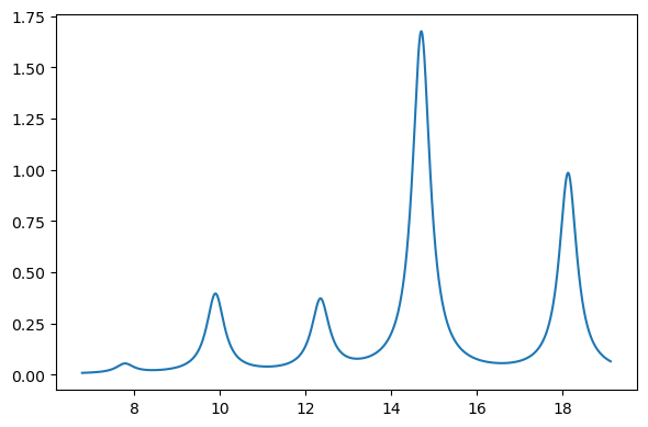
plt.figure(figsize=(6, 4))
x = au2ev * rpa_results["eigenvalues"]
y = rpa_results["oscillator_strengths"]
xi, yi = lorentzian(x, y, min(x) - 1.0, max(x) + 1.0, 0.01, 0.5)
plt.plot(xi, yi)
plt.tight_layout()
plt.show()
Energy [au]  Osc. str.   TM(x)     TM(y)     TM(z)
   0.286      0.01128  -0.00000   0.00000  -0.24321
   0.364      0.09652  -0.00000   0.63080  -0.00000
   0.364      0.00000   0.00000  -0.00000   0.00000
   0.454      0.08684  -0.53570  -0.00000  -0.00000
   0.540      0.41655  -1.07524   0.00000  -0.00000
   0.666      0.24377  -0.00000  -0.74073   0.00000
CPP-DFT#
Using CPP-DFT, the linear absorption cross-section is resolved over a range of energies, which is here chosen as the 7-17 eV (with a resolution of 0.1 eV):
Note
The frequency specification is currently being rewritten.
# Define spectrum region to be resolved
xmin, xmax = 7.0, 17.0
freqs = np.arange(xmin, xmax, 0.1) / au2ev
freqs_str = [str(x) for x in freqs]

# Calculate the response
cpp_drv = vlx.rsplinabscross.LinearAbsorptionCrossSection(
    {"frequencies": ",".join(freqs_str), "damping": 0.3 / au2ev}, method_settings
)
cpp_drv.init_driver()
cpp_results = cpp_drv.compute(molecule, basis, scf_results)

# Extract the imaginary part of the complex response function and convert to absorption cross section
sigma = []
for w in freqs:
    axx = -cpp_drv.rsp_property["response_functions"][("x", "x", w)].imag
    ayy = -cpp_drv.rsp_property["response_functions"][("y", "y", w)].imag
    azz = -cpp_drv.rsp_property["response_functions"][("z", "z", w)].imag
    alpha_bar = (axx + ayy + azz) / 3.0
    sigma.append(4.0 * np.pi * w * alpha_bar / 137.035999)
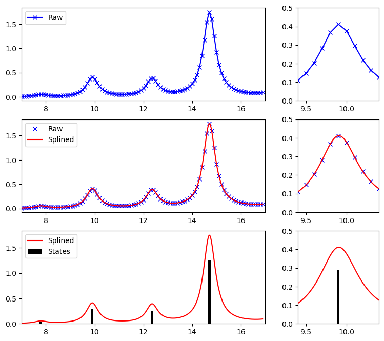
Plotting the raw output, the raw output with a splined function, and a comparison to the eigenstate results above (here plotted as bars):
# Make figure with panels of 3:1 width
plt.figure(figsize=(9, 8))
gs = gridspec.GridSpec(3, 2, width_ratios=[3, 1])

# Raw results for the full region
plt.subplot(gs[0])
plt.plot(au2ev * freqs, sigma, "bx-")
plt.legend(("Raw", ""), loc="upper left")
plt.xlim((xmin, xmax))

# Raw results for a zoomed in region
plt.subplot(gs[1])
plt.plot(au2ev * freqs, sigma, "bx-")
plt.xlim((9.4, 10.4))
plt.ylim((0, 0.50))

# Raw and splined spectra for the full region
plt.subplot(gs[2])
plt.plot(au2ev * freqs, sigma, "bx")
x = np.arange(min(au2ev * freqs), max(au2ev * freqs), 0.01)
y = interp1d(au2ev * freqs, sigma, kind="cubic")
plt.plot(x, y(x), "r")
plt.legend(("Raw", "Splined"), loc="upper left")
plt.xlim((xmin, xmax))

# Zoomed in raw and splined spectra
plt.subplot(gs[3])
plt.plot(au2ev * freqs, sigma, "bx")
plt.plot(x, y(x), "r")
plt.xlim((9.4, 10.4))
plt.ylim((0, 0.50))

# Zoomed in raw and splined spectra for the full region
plt.subplot(gs[4])
x = np.arange(min(au2ev * freqs), max(au2ev * freqs), 0.01)
y = interp1d(au2ev * freqs, sigma, kind="cubic")
plt.plot(x, y(x), "r")
xi = au2ev * rpa_results["eigenvalues"]
yi = rpa_results["oscillator_strengths"]
plt.bar(xi, 3.0 * yi, width=0.1, color="k")
plt.legend(("Splined", "States"), loc="upper left")
plt.xlim((xmin, xmax))

# Zoomed in raw and splined spectra
plt.subplot(gs[5])
plt.plot(x, y(x), "r")
plt.bar(xi, 3.0 * yi, width=0.025, color="k")
plt.xlim((9.4, 10.4))
plt.ylim((0, 0.50))

plt.show()
ADC#
The first six excited states of water is calculated as:
# Construct structure and basis objects
molecule = gator.get_molecule(water_mol_str)
basis = gator.get_molecular_basis(molecule, "6-31G")

# Perform SCF calculation
scf_gs = gator.run_scf(molecule, basis)

# Calculate the 6 lowest eigenstates
adc_results = gator.run_adc(molecule, basis, scf_gs, method="adc3", singlets=6)
The resuls can be printed as a table, and convoluted and plotted using built-in functionalities (which can use several different energy-axis, as shown below).
Note
The adc3 (adc2) designation from adc_results.describe() means that energies are calculated at an ADC(3) level, while properties are given at an ADC(2) level. This is sometimes referred to as ADC(3/2), as well.
# Print information on eigenstates
print(adc_results.describe())

# Plot using built-in functionalities
plt.figure(figsize=(10, 6))
plt.subplot(221)
plt.title("In eV")
adc_results.plot_spectrum(xaxis="eV")

plt.subplot(222)
plt.title("In atomic units")
adc_results.plot_spectrum(xaxis="au")

plt.subplot(223)
plt.title("In nm")
adc_results.plot_spectrum(xaxis="nm", broadening=None)

plt.subplot(224)
plt.title(r"In cm$^{-1}$")
adc_results.plot_spectrum(xaxis="cm-1")
plt.tight_layout()
plt.show()
+--------------------------------------------------------------+
| adc3 (adc2)                             singlet ,  converged |
+--------------------------------------------------------------+
|  #        excitation energy     osc str    |v1|^2    |v2|^2  |
|          (au)           (eV)                                 |
|  0     0.3127134      8.509364   0.0134     0.951   0.04895  |
|  1     0.3933877      10.70463   0.0000    0.9532   0.04681  |
|  2     0.4056694      11.03883   0.1161    0.9491   0.05091  |
|  3     0.4916579      13.37869   0.1103     0.949   0.05096  |
|  4     0.5655096       15.3883   0.4351    0.9625   0.03751  |
|  5     0.6977152       18.9858   0.2604    0.9537   0.04626  |
+--------------------------------------------------------------+
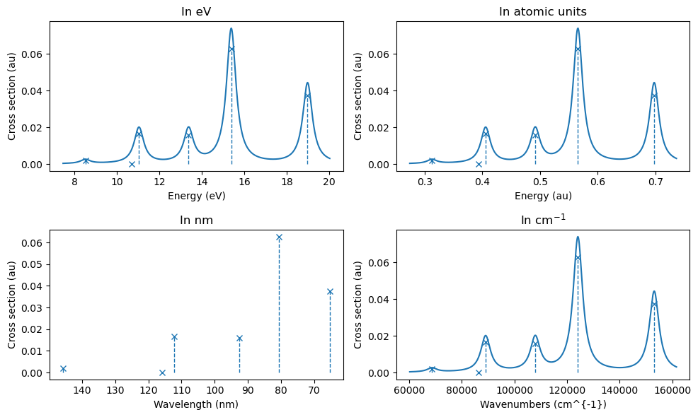
Fix: broaden spectra expressed in wavelength.
Note that some high-energy features can be the result of a discretized continuum region. A larger basis set will flatten out this region, but care should be taken for any analysis of that part of the spectrum.
CPP-ADC#
To be added.
MCSCF#
In some cases, it can be preferable to use a multiconfigurational wavefunction to compute excitation energies. This is necessary if, for instance, the molecule is suspected to have strong correlation effects, or if the user is interested in analyzing a conical intersection — something that ADC and TDDFT often fail to properly describe.
In principle, a MCSCF spectrum can be computed using response theory similarly to ADC and DFT. However, as configuration interaction (CI) can naturally provide not just the lowest but any state, it is possible to produce excited states by simply increasing the number of requested states or “roots” in the CI. However, in traditional MCSCF, the orbitals cannot be simultaneously optimized for each state, and instead we use a set of orbitals that is a compromise between all states: the state-averaged orbitals.
For water in its equilibrium distance, there is no strong correlation, and thus the only orbitals we need to include in the active space are those that can be excited in the UV-visible spectrum. Here, we will use a CASSCF with an active space comprising the molecular orbitals formed by the oxygen 2p and hydrogen 1s, corresponding to the two \(\sigma\) and \(\sigma^*\) and one oxygen lone pair. We could in principle include the other lone pair, formed mostly by the 2s orbital of the oxygen, but its orbital energy is much lower and the orbital is thus not involved in the lowest UV-visible transitions.
The orbitals are conveniently located around the HOMO-LUMO gap, so it is sufficient to request a CAS(6,5) (6 electrons in 5 orbitals) to get the desired active space. First, we calculate the SCF ground state:
# Prepare molecule and basis objects
molecule = vlx.Molecule.read_molecule_string(water_mol_str)
basis = vlx.MolecularBasis.read(molecule, "6-31G")

# SCF calculation
scf_drv = vlx.ScfRestrictedDriver()
scf_results = scf_drv.compute(molecule, basis)
Then we resolve the six lowest excited states:
# Active space settings
space = mtp.OrbSpace(molecule, scf_drv.mol_orbs)
space.cas(6, 5)  # 3 O_2p and 2 H_1s

# CASSCF calculation
mcscf_drv = mtp.McscfDriver()
mcscf_results = mcscf_drv.compute(molecule, basis, space, 6)

# Transition properties
SI = mtp.StateInteraction()
si_results = SI.compute(molecule, basis, mcscf_results)
Show code cell output
                          Multi-Configurational Self-Consistent Field Driver
                         ====================================================
               Active space definition:
               ------------------------
               Number of inactive (occupied) orbitals: 2
               Number of active orbitals:              5
               Number of virtual orbitals:             6

               This is a CASSCF wavefunction: CAS(6,5)

               CI expansion:
               -------------
               Number of determinants:      100


               ╭────────────────────────────────────╮
               │          Driver settings           │
               ╰────────────────────────────────────╯


               Number of states              :   6
               State-averaged calculation
                - Equal-weights
               Max. iterations               :   50
               BFGS window                   :   5
               Convergence thresholds:
                - Energy change              :   1e-08
                - Gradient sq. norm          :   1e-08


                          MCSCF Iterations
                         -------------------

     Iter. | Average Energy | E. Change | Grad. Norm | CI Iter. | Trust rad. |  Time
     ---------------------------------------------------------------------------------
1 -75.617648941 0.0e+00 9.7e-02 0 0.40 0:00:00
2 -75.642903350 -2.5e-02 1.4e-02 0 0.40 0:00:00
3 -75.646125925 -3.2e-03 1.6e-04 0 0.40 0:00:00
4 -75.646212175 -8.6e-05 3.4e-06 0 0.40 0:00:00
5 -75.646218727 -6.6e-06 5.4e-07 0 0.48 0:00:00
6 -75.646219045 -3.2e-07 1.8e-08 0 0.58 0:00:00
7 -75.646219063 -1.8e-08 9.0e-10 0 0.58 0:00:00
        8     -75.646219065    -1.9e-09      1.0e-10          0        0.69    0:00:00
** Convergence reached in 8 iterations
        9     -75.646219065    -5.3e-11      3.7e-12          0        0.69    0:00:00

               Final results
               -------------

* State 1
  - S^2    : 0.00  (multiplicity = 1.0 )
  - Energy : -75.98281062496535
  - Natural orbitals
1.98486 1.99960 1.99160 0.00851 0.01544

* State 2
  - S^2    : 0.00  (multiplicity = 1.0 )
  - Energy : -75.7040492619663
  - Natural orbitals
1.98828 1.00000 1.99728 0.99912 0.01531

* State 3
  - S^2    : -0.00  (multiplicity = 1.0 )
  - Energy : -75.62045138647319
  - Natural orbitals
1.99530 1.00000 1.99422 0.01264 0.99784

* State 4
  - S^2    : 0.00  (multiplicity = 1.0 )
  - Energy : -75.60225041976749
  - Natural orbitals
1.96141 1.99969 1.22263 0.77478 0.04148

* State 5
  - S^2    : 0.00  (multiplicity = 1.0 )
  - Energy : -75.52004110975051
  - Natural orbitals
1.97752 1.99960 1.01676 0.02746 0.97865

* State 6
  - S^2    : 0.00  (multiplicity = 1.0 )
  - Energy : -75.44771158728814
  - Natural orbitals
1.01935 1.99895 1.97785 0.97990 0.02395

                                                 Spin Restricted Orbitals
                                                 ------------------------

               Molecular Orbital No.   1:
               --------------------------
               Occupation: 2.000 Energy:  -20.68879 a.u.
               (   1 O   1s  :    -1.00)

               Molecular Orbital No.   2:
               --------------------------
               Occupation: 2.000 Energy:   -1.45143 a.u.
               (   1 O   1s  :     0.22) (   1 O   2s  :    -0.49) (   1 O   3s  :    -0.48)

               Molecular Orbital No.   3:
               --------------------------
               Occupation: 1.816 Energy:   -0.76930 a.u.
               (   1 O   1p+1:     0.56) (   1 O   2p+1:     0.29) (   2 H   1s  :    -0.23)
               (   3 H   1s  :     0.23)

               Molecular Orbital No.   4:
               --------------------------
               Occupation: 1.666 Energy:   -0.52443 a.u.
               (   1 O   1p0 :    -0.67) (   1 O   2p0 :    -0.48)

               Molecular Orbital No.   5:
               --------------------------
               Occupation: 1.666 Energy:   -0.59973 a.u.
               (   1 O   2s  :    -0.18) (   1 O   3s  :    -0.24) (   1 O   1p-1:    -0.60)
               (   1 O   2p-1:    -0.40)

               Molecular Orbital No.   6:
               --------------------------
               Occupation: 0.501 Energy:    0.10225 a.u.
               (   1 O   2s  :    -0.16) (   1 O   3s  :    -1.09) (   1 O   1p-1:     0.25)
               (   1 O   2p-1:     0.40) (   2 H   2s  :     0.94) (   3 H   2s  :     0.94)

               Molecular Orbital No.   7:
               --------------------------
               Occupation: 0.351 Energy:    0.21690 a.u.
               (   1 O   1p+1:    -0.42) (   1 O   2p+1:    -0.69) (   2 H   2s  :    -1.24)
               (   3 H   2s  :     1.24)

               Molecular Orbital No.   8:
               --------------------------
               Occupation: 0.000 Energy:    0.99875 a.u.
               (   1 O   2p+1:    -0.69) (   2 H   1s  :    -0.97) (   2 H   2s  :     0.59)
               (   3 H   1s  :     0.97) (   3 H   2s  :    -0.59)

               Molecular Orbital No.   9:
               --------------------------
               Occupation: 0.000 Energy:    1.06993 a.u.
               (   1 O   1p0 :    -0.94) (   1 O   2p0 :     1.05)
                                                Dipole moment for state 1
                                               ---------------------------

                                   X   :         0.000000 a.u.         0.000000 Debye
                                   Y   :        -0.848594 a.u.        -2.156911 Debye
                                   Z   :         0.000000 a.u.         0.000000 Debye
                                 Total :         0.848594 a.u.         2.156911 Debye
                                                Dipole moment for state 2
                                               ---------------------------

                                   X   :        -0.000000 a.u.        -0.000000 Debye
                                   Y   :         0.088075 a.u.         0.223865 Debye
                                   Z   :         0.000000 a.u.         0.000000 Debye
                                 Total :         0.088075 a.u.         0.223865 Debye
                                                Dipole moment for state 3
                                               ---------------------------

                                   X   :         0.000000 a.u.         0.000000 Debye
                                   Y   :        -0.019117 a.u.        -0.048591 Debye
                                   Z   :        -0.000000 a.u.        -0.000000 Debye
                                 Total :         0.019117 a.u.         0.048591 Debye
                                                Dipole moment for state 4
                                               ---------------------------

                                   X   :         0.000000 a.u.         0.000000 Debye
                                   Y   :         0.127030 a.u.         0.322878 Debye
                                   Z   :        -0.000000 a.u.        -0.000000 Debye
                                 Total :         0.127030 a.u.         0.322878 Debye
                                                Dipole moment for state 5
                                               ---------------------------

                                   X   :        -0.000000 a.u.        -0.000000 Debye
                                   Y   :         0.138716 a.u.         0.352582 Debye
                                   Z   :         0.000000 a.u.         0.000000 Debye
                                 Total :         0.138716 a.u.         0.352582 Debye
                                                Dipole moment for state 6
                                               ---------------------------

                                   X   :        -0.000000 a.u.        -0.000000 Debye
                                   Y   :        -0.255728 a.u.        -0.649995 Debye
                                   Z   :         0.000000 a.u.         0.000000 Debye
                                 Total :         0.255728 a.u.         0.649995 Debye
Total MCSCF time: 00:00:00
List of oscillator strengths greather than 1e-10

  From     to       Energy (eV)    Oscillator strength (length and velocity)
     1       2        7.58548         1.220177e-02    2.799370e-02
     1       4       10.35557         1.097829e-01    1.281789e-01
     1       5       12.59260         1.545515e-01    1.469851e-01
     1       6       14.56079         5.993553e-01    3.307390e-01

List of rotatory strengths greather than 1e-10

  From     to       Energy (eV)    Rot. strength (a.u. and 10^-40 cgs)
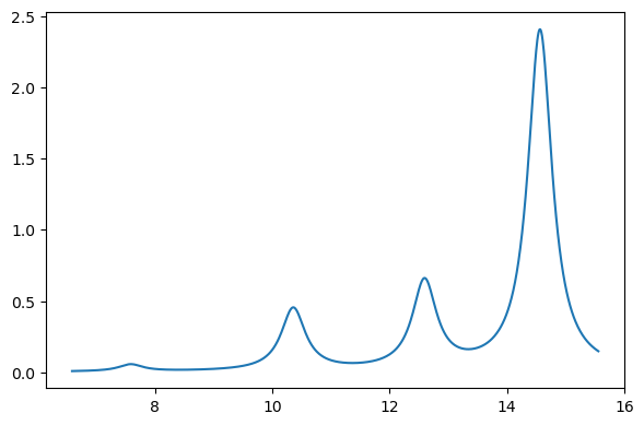
The resulting states are printed above, or can be printed or plotted:
# Print results as a table
print("Energy [au]  Osc. str.")
for i in np.arange(len(si_results["energies"])):
    e, os = (
        si_results["energies"][i],
        si_results["oscillator_strengths"][i],
    )
    print("   {:.3f}     {:8.5f}".format(e, os))

plt.figure(figsize=(6, 4))
x = au2ev * np.array(si_results["energies"])
y = si_results["oscillator_strengths"]
xi, yi = lorentzian(x, y, min(x) - 1.0, max(x) + 1.0, 0.01, 0.5)
plt.plot(xi, yi)
plt.tight_layout()
plt.show()
Energy [au]  Osc. str.
   0.279      0.01220
   0.362      0.00000
   0.381      0.10978
   0.463      0.15455
   0.535      0.59936
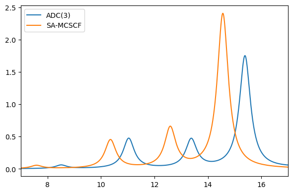
Comparing to ADC(3) we see a good agreement in relative features, but the absolute energies and intensities are a bit different:
plt.figure(figsize=(6, 4))

# ADC(3)
x, y = au2ev * adc_results.excitation_energy, adc_results.oscillator_strength
xi, yi = lorentzian(x, y, xmin, xmax, 0.01, 0.5)
plt.plot(xi, yi)

# SA-MCSCF
x = au2ev * np.array(si_results["energies"])
y = si_results["oscillator_strengths"]
xi, yi = lorentzian(x, y, xmin, xmax, 0.01, 0.5)
plt.plot(xi, yi)
plt.legend(("ADC(3)", "SA-MCSCF"))
plt.xlim((xmin, xmax))
plt.tight_layout()
plt.show()
Comparison of spectra#
The spectra from the four different approaches can be plotted as:
fig, (ax1, ax2) = plt.subplots(1, 2)
fig.set_figheight(4)
fig.set_figwidth(10)

xmin, xmax = 7, 17

# ADC(3)
x, y = au2ev * adc_results.excitation_energy, adc_results.oscillator_strength
xi, yi = lorentzian(x, y, xmin, xmax, 0.01, 0.5)
ax1.plot(xi, yi)
ax2.plot(xi, yi)

# TDDFT
x = au2ev * rpa_results["eigenvalues"]
y = rpa_results["oscillator_strengths"]
xi, yi = lorentzian(x, y, xmin, xmax, 0.01, 0.5)
ax1.plot(xi, yi)
ax2.plot(xi, yi + 1)

# SA-MCSCF
x = au2ev * np.array(si_results["energies"])
y = si_results["oscillator_strengths"]
xi, yi = lorentzian(x, y, xmin, xmax, 0.01, 0.5)
ax1.plot(xi, yi)
ax2.plot(xi, yi + 2)

ax1.legend(("ADC(3)", "TDDFT", "SA-MCSCF"))
ax1.set_xlim((xmin, xmax))
ax2.set_xlim((xmin, xmax))
plt.tight_layout()
plt.show()
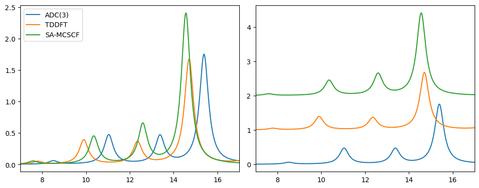
Plotted either on top of each other, or with a vertical set-off. We note that the features are, in general, similar, with differences mainly taking the form of absolute energy shifts, as well as noticeably more intense features for SA-MCSCF.