Exercises#
ADC summary#
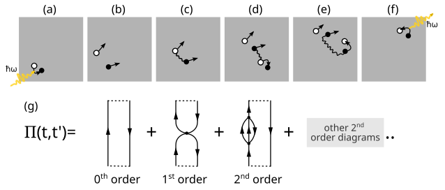
The poles and residues of the polarization propagator described by the spectral representation describe excitation energies and transition amplitudes, respectively. One possible strategy to determine these quantities is to expand \(\Pi_{pq,rs}\) in a time-dependent perturbation series based on a Hamiltonian partitioned in the same way as for the Møller\(-\)Plesset ground-state. This expansion is also called a diagrammatic expansion because each term in the series can be represented by a Feynman diagram (see figure above). The above equation can be regarded as the diagonal form of the polarization propagator, which, when considering only the first term and ignoring the broadening, can be written in matrix form as
or in non-diagonal form,
ISR for ADC(0) and ADC(1)#
The elements of the ADC matrix \(\mathbf{M}\) are obtained as matrix elements of the shifted Hamiltonian in the basis of the intermediate states,
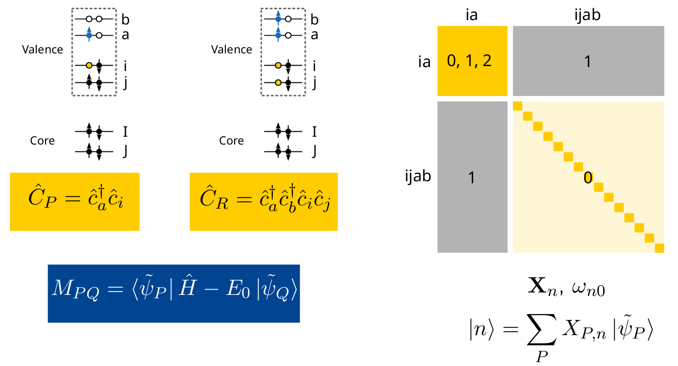
This representation of the shifted Hamiltonian leads to a Hermitian eigenvalue equation,
yielding vertical excitation energies (\(\omega_{n0} = E_n - E_0\)) and the corresponding excitation vectors \(\mathbf{X}_n\).
Expanding in series the ADC matrix elements in terms of the perturbation, explicit expressions are obtained,
In the following, we will construct the ADC(0) and ADC(1) matrices for the water molecule using a minimal basis set (STO-3G). This will allow us to visualize the entire matrices and obtain the eigenvalues and eigenvectors. The first step is to carry out a HF reference calculation to obtain the orbital eigenvalues and two electron repulsion integrals in MO basis required by the matrix elements above.
import veloxchem as vlx
import gator
import py3Dmol as p3d
import numpy as np
from veloxchem.mointsdriver import MOIntegralsDriver
from matplotlib import pyplot as plt
from matplotlib import colormaps
np.set_printoptions(precision=3, suppress=True)
# Conversion from Hartree to eV for later use
au2ev = vlx.veloxchemlib.hartree_in_ev()
lih_xyz = """2
Li 0.000000 0.000000 0.000000
H 0.000000 0.000000 1.000000
"""
water_xyz = """3
O 0.0000000000 0.0000000000 0.1178336003
H -0.7595754146 -0.0000000000 -0.4713344012
H 0.7595754146 0.0000000000 -0.4713344012
"""
name = "h2o"
molecule = vlx.Molecule.read_xyz_string(water_xyz)
basis_set_label = "sto-3g"
basis = vlx.MolecularBasis.read(molecule, basis_set_label)
Show code cell source
viewer = p3d.view(viewergrid=(1, 1), width=500, height=300)
viewer.addModel(water_xyz, 'xyz', viewer=(0, 0))
viewer.setViewStyle({"style": "outline", "width": 0.05})
viewer.setStyle({"stick":{},"sphere": {"scale":0.25}})
# viewer.rotate(90,'y')
viewer.rotate(-90,'x')
viewer.show()
3Dmol.js failed to load for some reason. Please check your browser console for error messages.
Step 1. Calculate the reference state#
# SCF will be run by VeloxChem through Gator
scf = gator.run_scf(molecule, basis, conv_thresh=1e-10, verbose=True)
Show code cell output
Self Consistent Field Driver Setup
====================================
Wave Function Model : Spin-Restricted Hartree-Fock
Initial Guess Model : Superposition of Atomic Densities
Convergence Accelerator : Two Level Direct Inversion of Iterative Subspace
Max. Number of Iterations : 50
Max. Number of Error Vectors : 10
Convergence Threshold : 1.0e-10
ERI Screening Threshold : 1.0e-12
Linear Dependence Threshold : 1.0e-06
* Info * Nuclear repulsion energy: 9.1561447194 a.u.
* Info * Overlap matrix computed in 0.00 sec.
* Info * Kinetic energy matrix computed in 0.00 sec.
* Info * Nuclear potential matrix computed in 0.00 sec.
* Info * Orthogonalization matrix computed in 0.00 sec.
* Info * Starting Reduced Basis SCF calculation...
* Info * ...done. SCF energy in reduced basis set: -74.963513321178 a.u. Time: 0.02 sec.
* Info * Overlap matrix computed in 0.00 sec.
* Info * Kinetic energy matrix computed in 0.00 sec.
* Info * Nuclear potential matrix computed in 0.00 sec.
* Info * Orthogonalization matrix computed in 0.00 sec.
Iter. | Hartree-Fock Energy | Energy Change | Gradient Norm | Max. Gradient | Density Change
--------------------------------------------------------------------------------------------
1 -74.963513323401 0.0000000000 0.00002852 0.00000681 0.00000000
2 -74.963513323651 -0.0000000002 0.00000905 0.00000208 0.00002371
3 -74.963513323683 -0.0000000000 0.00000065 0.00000015 0.00001205
4 -74.963513323684 -0.0000000000 0.00000002 0.00000000 0.00000042
5 -74.963513323684 0.0000000000 0.00000000 0.00000000 0.00000001
*** SCF converged in 5 iterations. Time: 0.02 sec.
Spin-Restricted Hartree-Fock:
-----------------------------
Total Energy : -74.9635133237 a.u.
Electronic Energy : -84.1196580431 a.u.
Nuclear Repulsion Energy : 9.1561447194 a.u.
------------------------------------
Gradient Norm : 0.0000000000 a.u.
Ground State Information
------------------------
Charge of Molecule : 0.0
Multiplicity (2S+1) : 1
Magnetic Quantum Number (M_S) : 0.0
Spin Restricted Orbitals
------------------------
Molecular Orbital No. 1:
--------------------------
Occupation: 2.000 Energy: -20.24239 a.u.
( 1 O 1s : -0.99)
Molecular Orbital No. 2:
--------------------------
Occupation: 2.000 Energy: -1.26646 a.u.
( 1 O 1s : 0.23) ( 1 O 2s : -0.83) ( 2 H 1s : -0.16)
( 3 H 1s : -0.16)
Molecular Orbital No. 3:
--------------------------
Occupation: 2.000 Energy: -0.61559 a.u.
( 1 O 1p+1: -0.61) ( 2 H 1s : 0.45) ( 3 H 1s : -0.45)
Molecular Orbital No. 4:
--------------------------
Occupation: 2.000 Energy: -0.45278 a.u.
( 1 O 2s : 0.54) ( 1 O 1p0 : 0.78) ( 2 H 1s : -0.28)
( 3 H 1s : -0.28)
Molecular Orbital No. 5:
--------------------------
Occupation: 2.000 Energy: -0.39107 a.u.
( 1 O 1p-1: 1.00)
Molecular Orbital No. 6:
--------------------------
Occupation: 0.000 Energy: 0.60182 a.u.
( 1 O 2s : 0.88) ( 1 O 1p0 : -0.74) ( 2 H 1s : -0.79)
( 3 H 1s : -0.79)
Molecular Orbital No. 7:
--------------------------
Occupation: 0.000 Energy: 0.73721 a.u.
( 1 O 1p+1: 0.99) ( 2 H 1s : 0.84) ( 3 H 1s : -0.84)
Ground State Dipole Moment
----------------------------
X : -0.000000 a.u. -0.000000 Debye
Y : -0.000000 a.u. -0.000000 Debye
Z : -0.677172 a.u. -1.721200 Debye
Total : 0.677172 a.u. 1.721200 Debye
# Let's have a look at the molecular orbitals
orb_viewer = vlx.OrbitalViewer()
orb_viewer.plot(molecule, basis, scf.mol_orbs)
Step 2. Construct the ADC(0) and ADC(1) matrices#
The ADC(0) matrix consists of only \(\mathbf{M}^{(0)}\) matrix elements, while the ADC(1) matrix is \(\mathbf{M} = \mathbf{M}^{(0)} + \mathbf{M}^{(1)}\). As discussed above and using spin-orbitals,
For a closed-shell restricted HF reference, \(M_{ia,jb}^{(1)}\) can be written in terms of spatial orbitals (in Chemist’s notation) as
Let’s extract the MO energies and two-electron integrals:
# MO energies in diagonal matrix
mo_energies = np.diag(scf.scf_tensors['E_alpha'])
# Two-electron integrals from vlx
moints_drv = MOIntegralsDriver()
oovv = moints_drv.compute_in_memory(molecule, basis, scf.mol_orbs, "chem_OOVV")
ovov = moints_drv.compute_in_memory(molecule, basis, scf.mol_orbs, "chem_OVOV")
Construct the ADC matrices:
# Number of occupied and virtual orbitals
nocc = molecule.number_of_alpha_electrons()
norb = mo_energies.shape[0]
nvir = norb - nocc
nexc = nocc * nvir # number of excited (singlet or triplet) states in ADC(1)
print("nocc: ", nocc)
print("nvir: ", nvir)
# ADC matrices with zeroes
adc0_mat4d = np.zeros((nocc, nvir, nocc, nvir))
adc1_mat4d = np.zeros((nocc, nvir, nocc, nvir))
# Loop over all indices and fill matrix with corresponding elements
for i in range(nocc):
for a in range(nvir):
# Fill the diagonal (orbital-energy differences)
adc0_mat4d[i,a,i,a] = ...
adc1_mat4d[i,a,i,a] = ...
for j in range(nocc):
for b in range(nvir):
# Fill the rest (two-electron integrals)
...
...
Show code cell content
# Number of occupied and virtual orbitals
nocc = molecule.number_of_alpha_electrons()
norb = mo_energies.shape[0]
nvir = norb - nocc
nexc = nocc * nvir # number of excited (singlet or triplet) states in ADC(1)
print("nocc: ", nocc)
print("nvir: ", nvir)
# ADC matrices with zeroes
adc0_mat4d = np.zeros((nocc, nvir, nocc, nvir))
adc1_mat4d = np.zeros((nocc, nvir, nocc, nvir))
# Loop over all indices and fill matrix with corresponding elements
for i in range(nocc):
for a in range(nvir):
# Fill the diagonal (orbital-energy differences)
adc0_mat4d[i,a,i,a] = mo_energies[nocc+a,nocc+a] - mo_energies[i,i]
adc1_mat4d[i,a,i,a] = mo_energies[nocc+a,nocc+a] - mo_energies[i,i]
for j in range(nocc):
for b in range(nvir):
# Fill the rest (two-electron integrals)
adc1_mat4d[i,a,j,b] -= oovv[i,j,a,b] #ovov[j,a,i,b]
adc1_mat4d[i,a,j,b] += 2 * ovov[i,a,j,b] #2*oovv[i,j,a,b]
nocc: 5
nvir: 2
Reshape into 2D matrices:
# Reshape the 4D into 2D matrices
adc0_mat2d = adc0_mat4d.reshape((nocc*nvir, nocc*nvir))
print("closed-shell ADC(0) matrix:\n", adc0_mat2d.shape, "\n", adc0_mat2d)
adc1_mat2d = adc1_mat4d.reshape((nocc*nvir, nocc*nvir))
print("\nclosed-shell ADC(1) matrix:\n", adc1_mat2d.shape, "\n", adc1_mat2d)
Show code cell output
closed-shell ADC(0) matrix:
(10, 10)
[[20.844 0. 0. 0. 0. 0. 0. 0. 0. 0. ]
[ 0. 20.98 0. 0. 0. 0. 0. 0. 0. 0. ]
[ 0. 0. 1.868 0. 0. 0. 0. 0. 0. 0. ]
[ 0. 0. 0. 2.004 0. 0. 0. 0. 0. 0. ]
[ 0. 0. 0. 0. 1.217 0. 0. 0. 0. 0. ]
[ 0. 0. 0. 0. 0. 1.353 0. 0. 0. 0. ]
[ 0. 0. 0. 0. 0. 0. 1.055 0. 0. 0. ]
[ 0. 0. 0. 0. 0. 0. 0. 1.19 0. 0. ]
[ 0. 0. 0. 0. 0. 0. 0. 0. 0.993 0. ]
[ 0. 0. 0. 0. 0. 0. 0. 0. 0. 1.128]]
closed-shell ADC(1) matrix:
(10, 10)
[[20.104 -0. 0.021 0. -0. -0.023 -0.022 -0. 0. -0. ]
[-0. 20.154 0. 0.046 -0.001 0. -0. -0.03 -0. 0. ]
[ 0.021 0. 1.458 -0. 0. 0.055 0.064 -0. -0. 0. ]
[ 0. 0.046 -0. 1.504 -0.028 -0. -0. -0.019 -0. 0. ]
[-0. -0.001 0. -0.028 0.788 0. 0. 0.041 0. -0. ]
[-0.023 0. 0.055 -0. 0. 1.048 0.11 -0. -0. 0. ]
[-0.022 -0. 0.064 -0. 0. 0.11 0.644 -0. -0. 0. ]
[-0. -0.03 -0. -0.019 0.041 -0. -0. 0.721 0. -0. ]
[ 0. -0. -0. -0. 0. -0. -0. 0. 0.481 -0. ]
[-0. 0. 0. 0. -0. 0. 0. -0. -0. 0.552]]
Step 3. Diagonalize the ADC matrix#
# Diagonalize the ADC(1) matrix using numpy
adc0_eigvals, adc0_eigvecs = ...
adc1_eigvals, adc1_eigvecs = ...
np.set_printoptions(precision=2, suppress=True)
print("Closed-shell ADC(0) eigenvalues (H):\n", adc0_eigvals)
print()
print("Closed-shell ADC(0) eigenvalues (eV):\n", adc0_eigvals * au2ev)
print()
print("Closed-shell ADC(1) eigenvalues (eV):\n", adc1_eigvals * au2ev)
np.set_printoptions(precision=3, suppress=True)
Show code cell content
# Diagonalize the ADC(1) matrix using numpy
adc0_eigvals, adc0_eigvecs = np.linalg.eigh(adc0_mat2d)
adc1_eigvals, adc1_eigvecs = np.linalg.eigh(adc1_mat2d)
np.set_printoptions(precision=2, suppress=True)
print("Closed-shell ADC(0) eigenvalues (H):\n", adc0_eigvals)
print()
print("Closed-shell ADC(0) eigenvalues (eV):\n", adc0_eigvals * au2ev)
print()
print("Closed-shell ADC(1) eigenvalues (eV):\n", adc1_eigvals * au2ev)
np.set_printoptions(precision=3, suppress=True)
Closed-shell ADC(0) eigenvalues (H):
[ 0.99 1.05 1.13 1.19 1.22 1.35 1.87 2. 20.84 20.98]
Closed-shell ADC(0) eigenvalues (eV):
[ 27.02 28.7 30.7 32.38 33.13 36.81 50.84 54.52 567.2 570.88]
Closed-shell ADC(1) eigenvalues (eV):
[ 13.09 15.03 16.7 19.07 21.94 28.96 40.07 40.97 547.07 548.43]
The absorption spectrum#
In order to simulate a UV/vis or X-ray spectra, apart from the excitation energies also the spectral intensities are required. These are related to the absorption cross-sections and oscillator strengths. The oscillator strengths are obtained from the transition dipole moments. In order to obtain the latter, the ground- to excited-state one-particle transition density matrix is required,
where a transition matrix element was defined as, $\( \gamma_{pq} = \langle 0 | \hat{a}^\dagger_p\hat{a}_q | n\rangle = \sum_I \langle 0 | \hat{a}^\dagger_p\hat{a}_q | \tilde{\psi}_I \rangle x_I \)$
Through first order in perturbation theory, the non-vanishing part is given by
where the \(t\)-amplitudes are
The transition dipole moment \(T_{m}\) for the component \(m \in \{ x,y,z \}\) is obtained by contracting the transition density matrix with the corresponding dipole integrals \(\mu_{ia}^{m}\),
and the dimensionless oscillator strength \(f\), commonly used for relative intensities in the simulation of electronic spectra, is obtained from quantities in atomic units as
where \(\omega\) is the excitation energy of the corresponding excited state.
Note
In the CIS scheme, \(\gamma_{ia} = x_{ia}\) is correct through zeroth order only. As a matter of fact, this is the only place where the ADC(1) and CIS methods differ.
Let’s use the excitation vectors to build the one-particle transition density matrices and calculate the oscillator strengths.
We must first get the t-amplitudes,
# First, we need the t2-amplitudes
def get_t_amplitudes(molecule, basis, scf_drv):
#t_aaaa, t_abab, t_abba
#t_bbbb, t_baba, t_baab
scf_results = scf_drv.scf_tensors
N_O = molecule.number_of_alpha_electrons()
# extract the occupied subset of the orbital energies
e_occ = scf_results["E_alpha"][:N_O]
# extract the virtual subset of the orbital energies
e_vir = scf_results["E_alpha"][N_O:]
N_V = e_vir.shape[0]
# orbital energies and oovv integrals (spatial MO basis, physicists' notation)
# we use physicists notation here, as it is more convenient from the algorithm point of view
moeridrv = vlx.MOIntegralsDriver()
oovv = moeridrv.compute_in_memory(molecule, basis, mol_orbs=scf_drv.mol_orbs, moints_name="phys_OOVV")
e_ab = e_vir + e_vir.reshape(-1, 1) # epsilon_a + epsilon_b (as 2D matrix)
# Different spin blocks (a=alpha, b=beta)
t2_aaaa = np.zeros((N_O, N_O, N_V, N_V))
t2_abab = np.zeros((N_O, N_O, N_V, N_V))
t2_abba = np.zeros((N_O, N_O, N_V, N_V))
for i in range(N_O):
for j in range(N_O):
t2_aaaa[i,j] = (oovv[i, j] - oovv[i, j].T) / (e_ab - e_occ[i] - e_occ[j])
t2_abab[i,j] = (oovv[i, j]) / (e_ab - e_occ[i] - e_occ[j])
t2_abba[j,i] = (- oovv[j, i].T) / (e_ab - e_occ[i] - e_occ[j])
t2_mp2 = {'aaaa': t2_aaaa, 'abab': t2_abab, 'abba': t2_abba}
return t2_mp2
adc0_tdms = []
adc1_tdms = []
cis_tdms = []
t2_dict = get_t_amplitudes(molecule, basis, scf)
mo_occ = scf.scf_tensors['C_alpha'][:, :nocc]
mo_vir = scf.scf_tensors['C_alpha'][:, nocc:]
n_states = len(adc0_eigvals)
sqrt2 = np.sqrt(2)
for i in range(n_states):
# take just alpha-alpha part of the vector
# we need to divide by sqrt of 2.
x0 = 1/sqrt2 * adc0_eigvecs[:, i].reshape(nocc, nvir)
x1 = 1/sqrt2 * adc1_eigvecs[:, i].reshape(nocc, nvir)
# transform to AO basis, and sum alpha + beta
gamma_adc0 = np.linalg.multi_dot([mo_occ, x0, mo_vir.T])
gamma_adc0 += np.linalg.multi_dot([mo_vir, x0.T, mo_occ.T])
t_term = -np.einsum('jb,ijab->ia', x1, t2_dict['aaaa'])
t_term += -np.einsum('jb,ijab->ia', x1, t2_dict['abab'])
gamma_adc1 = np.linalg.multi_dot([mo_occ, x1 + t_term, mo_vir.T])
gamma_adc1 += np.linalg.multi_dot([mo_vir, (x1 + t_term).T, mo_occ.T])
gamma_cis = np.linalg.multi_dot([mo_occ, x1, mo_vir.T])
gamma_cis += np.linalg.multi_dot([mo_vir, x1.T, mo_occ.T])
cis_tdms.append(gamma_cis)
adc0_tdms.append(gamma_adc0)
adc1_tdms.append(gamma_adc1)
# Now we need to import the dipole moment integrals
# Dipole integrals in AO basis
dipole_drv = vlx.veloxchemlib.ElectricDipoleIntegralsDriver()
dipole_mats = dipole_drv.compute(molecule, basis)
dipole_ints_ao = np.array((dipole_mats.x_to_numpy(), dipole_mats.y_to_numpy(),
dipole_mats.z_to_numpy()))
Now we have all the ingredients to calculate the transition dipole moments and oscillator strengths.
adc0_osc_str = []
adc1_osc_str = []
cis_osc_str = []
for i in range(n_states):
tdm0 = ...
tdm1 = ...
tdm_cis =...
f0 = ...
f1 = ...
f_cis = ...
adc0_osc_str.append(f0)
adc1_osc_str.append(f1)
cis_osc_str.append(f_cis)
Show code cell content
adc0_osc_str = []
adc1_osc_str = []
cis_osc_str = []
for i in range(n_states):
tdm0 = np.einsum('xmn,mn->x', dipole_ints_ao, adc0_tdms[i])
tdm1 = np.einsum('xmn,mn->x', dipole_ints_ao, adc1_tdms[i])
tdm_cis = np.einsum('xmn,mn->x', dipole_ints_ao, cis_tdms[i])
f0 = 2.0/3.0 * adc0_eigvals[i] * np.linalg.norm(tdm0)**2
f1 = 2.0/3.0 * adc1_eigvals[i] * np.linalg.norm(tdm1)**2
f_cis = 2.0/3.0 * adc1_eigvals[i] * np.linalg.norm(tdm_cis)**2
adc0_osc_str.append(f0)
adc1_osc_str.append(f1)
cis_osc_str.append(f_cis)
In order to plot, we add a Lorentzian (or Gaussian) broadening to the spectra. A routine is provided below.
Show code cell source
def add_broadening(xb, yb, gamma=0.1, step=0.1, line_profile="lorentzian", sort=True):
""" Adds a Gaussian or Lorentizan broadening to a bar graph.
:param xb: the numpy array of energies.
:param yb: the numpy array of intensities.
:param gamma: the FWHM or HWHM.
:param step: the step size.
:param line_profile: the type of line profile (gaussian, or lorentzian).
returns two numpy arrays with the broadened energies and intensities.
"""
if sort:
for i in range(xb.shape[0]-1):
for j in range(i+1, xb.shape[0]):
if xb[i] > xb[j]:
xb_move = xb[i].copy()
yb_move = yb[i].copy()
xb[i] = xb[j].copy()
xb[j] = xb_move.copy()
yb[i] = yb[j].copy()
yb[j] = yb_move.copy()
x_min = xb[0] - 5 # in eV
x_max = xb[-1] + 5
x = np.arange(x_min, x_max, step)
y = np.zeros_like(x)
# go through the frames and calculate the spectrum for each frame
for i in range(x.shape[0]):
for e, f in zip(xb, yb):
if line_profile == 'gaussian':
y[i] += f * np.exp(-((e - x[i]) / gamma)**2)
elif line_profile == 'lorentzian':
y[i] += 0.5 * gamma * f / (np.pi * (
(x[i] - e)**2 + 0.25 * gamma**2))
return x, y
x_adc0, y_adc0 = add_broadening(np.array(adc0_eigvals)*au2ev, adc0_osc_str, step=0.05, gamma=0.4, sort=False)
x_adc1, y_adc1 = add_broadening(np.array(adc1_eigvals)*au2ev, adc1_osc_str, step=0.05, gamma=0.4, sort=False)
x_cis, y_cis = add_broadening(np.array(adc1_eigvals)*au2ev, cis_osc_str, step=0.05, gamma=0.4, sort=False)
Show code cell source
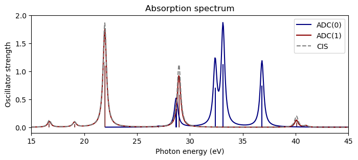
plt.figure(figsize=(8,3))
plt.bar(np.array(adc0_eigvals)*au2ev, adc0_osc_str, width=0.1, color="navy")
plt.bar(np.array(adc1_eigvals)*au2ev, adc1_osc_str, width=0.1, color="darkred")
plt.bar(np.array(adc1_eigvals)*au2ev, cis_osc_str, width=0.05, color="gray")
plt.plot(x_adc0, y_adc0, color="navy", label="ADC(0)")
plt.plot(x_adc1, y_adc1, color="darkred", label="ADC(1)")
plt.plot(x_cis, y_cis, "--", color="gray", label="CIS")
plt.xlim(15, 45)
plt.ylim(-0.1, 2.0)
plt.xlabel("Photon energy (eV)")
plt.ylabel("Oscillator strength")
plt.title("Absorption spectrum")
plt.legend()
plt.show()
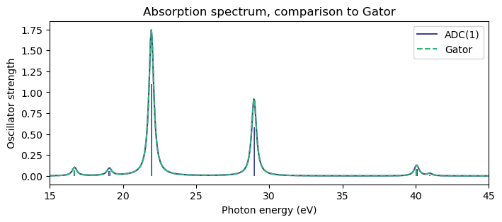
# Compare to Gator
adc1_results = gator.run_adc(molecule, basis, scf, verbose=False, method='adc1',
singlets=nexc, tol=1e-5)
/Users/evitols/miniconda3/envs/echem/lib/python3.12/site-packages/adcc/misc.py:26: UserWarning: pkg_resources is deprecated as an API. See https://setuptools.pypa.io/en/latest/pkg_resources.html. The pkg_resources package is slated for removal as early as 2025-11-30. Refrain from using this package or pin to Setuptools<81.
from pkg_resources import parse_version
Starting adc1 singlet Jacobi-Davidson ...
Niter n_ss max_residual time Ritz values
1 10 1.3766e-28 77ms [0.481 0.552 0.614 0.701 0.806 1.064 1.473]
=== Converged ===
Number of matrix applies: 10
Total solver time: 89.402ms
x_gator, y_gator = add_broadening(np.array(adc1_results.excitation_energy)*au2ev, adc1_results.oscillator_strength, step=0.05, gamma=0.4, sort=False)
print("Gator ADC(1) eigenvalues:")
print(adc1_results.excitation_energy)
print()
print("Our ADC(1) eigenvalues:")
print(adc1_eigvals)
Gator ADC(1) eigenvalues:
[ 0.481 0.552 0.614 0.701 0.806 1.064 1.473 1.506 20.104 20.154]
Our ADC(1) eigenvalues:
[ 0.481 0.552 0.614 0.701 0.806 1.064 1.473 1.506 20.104 20.154]
print("Gator ADC(1) oscillator strengths:")
print(adc1_results.oscillator_strength)
print()
print("Our ADC(1) oscillator strengths:")
print(np.array(adc1_osc_str))
print("\nCIS:")
print(np.array(cis_osc_str))
Gator ADC(1) oscillator strengths:
[0.003 0. 0.063 0.054 1.095 0.581 0.08 0.018 0.052 0.087]
Our ADC(1) oscillator strengths:
[0.003 0. 0.063 0.054 1.095 0.581 0.08 0.018 0.052 0.087]
CIS:
[0.004 0. 0.077 0.058 1.169 0.705 0.125 0.016 0.054 0.087]
cmap = colormaps['viridis']
Show code cell source
plt.figure(figsize=(8,3))
plt.bar(np.array(adc1_eigvals)*au2ev, adc1_osc_str, width=0.1, color=cmap(0.2))
plt.bar(np.array(adc1_results.excitation_energy)*au2ev, adc1_results.oscillator_strength, width=0.05, color=cmap(0.65))
plt.plot(x_adc1, y_adc1, color=cmap(0.2), label="ADC(1)")
plt.plot(x_gator, y_gator, '--', color=cmap(0.65), label="Gator")
#plt.plot(x_cis, y_cis, "--", color="gray", label="CIS")
plt.xlim(15, 45)
plt.ylim(-0.1, 1.85)
plt.xlabel("Photon energy (eV)")
plt.ylabel("Oscillator strength")
plt.title("Absorption spectrum, comparison to Gator")
plt.legend()
plt.show()
Excited state analysis#
It is very useful to further analyze the absorption spectrum and determine the nature of the excited state. For this purpose, the state density matrix (or rather the difference density matrix) can be partitioned in various ways. A particularly useful way is into attachment and detachment densities. By diagonalizing the attachment and detachment densities we can also calculate the so-called promotion numbers, i.e. the number of detached and attached electrons involved in the transition.
Attachment and detachment densities#
Attachment and detachment densities can be obtained by diagonalizing the difference density matrix (i.e. the difference between the initial and final state densities). See F. Plasser, M. Wormit, and A. Dreuw, J. Chem. Phys. 141, 024106 (2014)
The attachment density is constructed considering only the positive eigenvalues, while the detachment density considering only the negative eigenvalues $\(a_i = \max(\kappa_i, 0)\)\( \)\(\boldsymbol{\gamma_a} = \mathbf{W}^{\mathrm{T}}(\mathbf{a}\mathbb{1})\mathbf{W}\)$
The one-particle state density matrices, can be identified by formally writing the excited state energy as $\( E_n = \sum_{p,q}\gamma_{pq}f_{pq} + \frac14\sum_{pqrs}\Gamma_{pqrs}\langle pq||rs\rangle \)$
In the case of ADC(1), the energy of the n\(\mathrm{th}\) excited state is:
The state density matrix is then obtained by identifying the terms between the two equations above. The difference density matrix is simply the difference between the state density and the ground state density matrix. For both ADC(0) and ADC(1), the difference density has two non-zero blocks, calculated as,
Promotion numbers#
The integrals over space of the corresponding attachment and detachment densities give the “promotion numbers” (how many electrons are involved in the transition). These are calculated as, $\(p_A = \mathrm{Tr}(\boldsymbol{\gamma_a}) = \sum_i a_i\)\( \)\(p_D = \mathrm{Tr}(\boldsymbol{\gamma_d}) = \sum_i d_i\)$
Let’s write a routine to calculate the difference density matrix.
def calculate_difference_density(x, nocc, nvir):
""" Calculates the difference density matrix.
:param x: the excitation vector.
:param nocc: the number of occupied orbitals.
:param nvir: the number of virtual orbitals.
"""
ddm_mo = np.zeros((nocc+nvir, nocc+nvir))
ddm_mo[:nocc, :nocc] = ...
ddm_mo[nocc:, nocc:] = ...
return ddm_mo
Show code cell source
def calculate_difference_density(x, nocc, nvir):
""" Calculates the difference density matrix.
:param x: the excitation vector.
:param nocc: the number of occupied orbitals.
:param nvir: the number of virtual orbitals.
"""
ddm_mo = np.zeros((nocc+nvir, nocc+nvir))
ddm_mo[:nocc, :nocc] = -np.einsum('ia,ja->ij', x, x)
ddm_mo[nocc:, nocc:] = np.einsum('ia,ib->ab', x, x)
return ddm_mo
def get_attachement_detachement(density_mo, density_ao):
# Symmetrize the density matrix
# new_density = 0.5*( density + density.T)
k, w = np.linalg.eigh(density_mo)
k_ao, w_ao = np.linalg.eigh(density_ao)
k_detach = k.copy()
k_ao_d = k_ao.copy()
k_attach = k.copy()
k_ao_a = k_ao.copy()
# Detachment: set positive eigenvalues to 0
k_detach[k > 0] = 0
k_ao_d[ k_ao > 0] = 0
# Attachment: set negative eigenvalues to 0
k_attach[k < 0] = 0
k_ao_a[k_ao < 0] = 0
# Back-transform with numpy
detach_mo = w @ np.diag(k_detach) @ w.T
attach_mo = w @ np.diag(k_attach) @ w.T
detach_ao = w_ao @ np.diag(k_ao_d) @ w_ao.T
attach_ao = w_ao @ np.diag(k_ao_a) @ w_ao.T
return detach_ao, attach_ao, np.sum(k_detach), np.sum(k_attach)
Now we can use the VeloxChem visualization driver to obtain the attachment and detachment densities from the density matrices.
p_a = []
p_d = []
mo_coeff = scf.scf_tensors['C_alpha']
vis_drv = vlx.VisualizationDriver()
cube_points = [40, 40, 40]
cubic_grid = vis_drv.gen_cubic_grid(molecule, cube_points)
for i in range(n_states):
x = adc1_eigvecs[:, i].reshape(nocc, nvir)
density_mo = calculate_difference_density(x, nocc, nvir)
density_ao = np.linalg.multi_dot([mo_coeff, density_mo, mo_coeff.T])
# get the detachment and attachment densities in AO basis, as well as
# the promotion numbers.
detach_adc1, attach_adc1, pd, pa = get_attachement_detachement(density_mo, density_ao)
print("S%d. %.2f detached & %.2f attached electrons." % (i+1, pd, pa))
# C-object necessary to write the densities to a cube file
dens_DA = vlx.veloxchemlib.AODensityMatrix([detach_adc1, attach_adc1], vlx.veloxchemlib.denmat.rest)
detach_cube_name = name + "_adc1_S%d_detach.cube" % (i+1)
attach_cube_name = name + "_adc1_S%d_attach.cube" % (i+1)
print("\nWriting cube files:... ", attach_cube_name, detach_cube_name)
print()
# Use the visualization driver to write the attachment and detachment densities to cube files
vis_drv.compute(cubic_grid, molecule, basis, dens_DA, 0, 'alpha')
vis_drv.write_data(detach_cube_name, cubic_grid, molecule,
'detachment', 0, 'alpha')
vis_drv.compute(cubic_grid, molecule, basis, dens_DA, 1, 'alpha')
vis_drv.write_data(attach_cube_name, cubic_grid, molecule,
'attachment', 1, 'alpha')
# Now let's have a look at these densities
index = 5 # index of the excited state
isoval_d = 0.001
isoval_a = 0.001
Show code cell source
print(" Detachment density Attachment density")
print()
viewer = p3d.view(linked=True, viewergrid=(1, 2), width=800, height=300)
folder = "../../data/adc/"
name_d = folder + name + "_adc1_S%d_detach.cube" % (index)
name_a = folder + name + "_adc1_S%d_attach.cube" % (index)
# Detachment density
with open(name_d, "r") as f:
cube = f.read()
# Plot molecule and density structures
viewer.addModel(cube, "cube", viewer=(0, 0))
viewer.setStyle({"stick": {}, "sphere": {"scale":0.25}}, viewer=(0, 0))
# Negative and positive nodes
viewer.addVolumetricData(
cube, "cube", {"isoval": -isoval_d, "color": "blue", "opacity": 0.75}, viewer=(0, 0)
)
viewer.addVolumetricData(
cube, "cube", {"isoval": isoval_d, "color": "red", "opacity": 0.75}, viewer=(0, 0)
)
# Attachment density
with open(name_a, "r") as f:
cube = f.read()
# Plot molecule and density structures
viewer.addModel(cube, "cube", viewer=(0, 1))
viewer.setStyle({"stick": {}, "sphere": {"scale":0.25}}, viewer=(0, 1))
# Negative and positive nodes
viewer.addVolumetricData(
cube, "cube", {"isoval": -isoval_a, "color": "blue", "opacity": 0.75}, viewer=(0, 1)
)
viewer.addVolumetricData(
cube, "cube", {"isoval": isoval_a, "color": "red", "opacity": 0.75}, viewer=(0, 1)
)
viewer.rotate(-90,'x')
viewer.show()
x = adc1_eigvecs[:, index-1].reshape(nocc, nvir)
print("Energy and oscillator strength: %.2f eV, %.5f." % (adc1_eigvals[index-1]*au2ev, adc1_osc_str[index-1]))
print()
txt = " "
for a in range(nvir):
txt += " Vir %d " % (a + 1)
print(txt+"\n")
for i in range(nocc):
txt = "Occ %d: " % (i + 1)
for a in range(nvir):
txt += "%9.3f " % x[i,a]
print(txt)
#print(x)
Detachment density Attachment density
3Dmol.js failed to load for some reason. Please check your browser console for error messages.
Energy and oscillator strength: 21.94 eV, 1.09469.
Vir 1 Vir 2
Occ 1: -0.000 -0.001
Occ 2: -0.000 -0.048
Occ 3: -0.904 0.000
Occ 4: -0.000 -0.425
Occ 5: -0.000 0.000