Spectrum broadening#
In this section we will discuss the broadening of calculated spectra, and how they compare to the different broadening mechanisms of experimental measurements. As an example, we will consider the valence spectrum of water, calculated as:
import matplotlib.pyplot as plt
import numpy as np
import veloxchem as vlx

au2ev = 27.2113245

water_xyz = """3

O       0.0000000000     0.1178336003     0.0000000000
H      -0.7595754146    -0.4713344012     0.0000000000
H       0.7595754146    -0.4713344012     0.0000000000
"""

# Prepare molecule and basis objects
molecule = vlx.Molecule.read_xyz_string(water_xyz)
basis = vlx.MolecularBasis.read(molecule, "6-31G")
3Dmol.js failed to load for some reason. Please check your browser console for error messages.
# SCF settings and calculation
scf_drv = vlx.ScfRestrictedDriver()
scf_settings = {"conv_thresh": 1.0e-6}
method_settings = {"xcfun": "b3lyp"}
scf_drv.update_settings(scf_settings, method_settings)
scf_results = scf_drv.compute(molecule, basis)

# resolve four eigenstates
rpa_solver = vlx.lreigensolver.LinearResponseEigenSolver()
rpa_solver.update_settings({"nstates": 6}, method_settings)
rpa_results = rpa_solver.compute(molecule, basis, scf_results)
With excited state energies, oscillator strengths, and transition moments:
print("Energy [au]  Osc. str.   TM(x)     TM(y)     TM(z)")
for i in np.arange(len(rpa_results["eigenvalues"])):
    e, os, x, y, z = (
        rpa_results["eigenvalues"][i],
        rpa_results["oscillator_strengths"][i],
        rpa_results["electric_transition_dipoles"][i][0],
        rpa_results["electric_transition_dipoles"][i][1],
        rpa_results["electric_transition_dipoles"][i][2],
    )
    print("   {:.3f}     {:8.5f}  {:8.5f}  {:8.5f}  {:8.5f}".format(e, os, x, y, z))
Energy [au]  Osc. str.   TM(x)     TM(y)     TM(z)
   0.286      0.01128   0.00000  -0.00000   0.24321
   0.364      0.09652  -0.00000  -0.63080   0.00000
   0.364      0.00000   0.00000   0.00000  -0.00000
   0.454      0.08684  -0.53570   0.00000  -0.00000
   0.540      0.41655  -1.07524  -0.00000   0.00000
   0.666      0.24377   0.00000  -0.74073   0.00000
Broadening in experiment#
The line shape of an experimental spectrum is affected by a number of factors, including:
Resolution of measurement
Vibrational effects
These leads to a number of different broadening types, such as
Lorentzian (homogenous?)
From life-time broadeningGaussian (inhomogenous?)
From Doppler broadening and resolution of measurementVoigt
A convolution of a Gaussian and a LorentzianAsymmetric
From vibrational effects
Lorentzian#
Cauchy distribution \(f\)
with FWHM of \(2\gamma_k\). This is normalized
Amplitude \(1/(\gamma \pi)\).
Gaussian#
HWHM is \(\sigma \sqrt{\textrm{ln 2}}/{\sqrt{2}}\)
Voigt#
Broadening calculated spectrum#
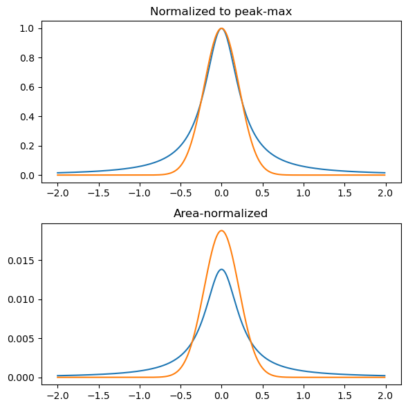
Considering only a single feature, a Lorentzian and Gaussian convolution leads to features:
def lorentzian(x, y, xmin, xmax, xstep, gamma):
    xi = np.arange(xmin, xmax, xstep)
    yi = np.zeros(len(xi))
    for i in range(len(xi)):
        for k in range(len(x)):
            yi[i] = (
                yi[i]
                + y[k] * gamma / ((xi[i] - x[k]) ** 2 + (gamma / 2.0) ** 2) / np.pi
            )
    return xi, yi


def gaussian(x, y, xmin, xmax, xstep, sigma):
    xi = np.arange(xmin, xmax, xstep)
    yi = np.zeros(len(xi))
    for i in range(len(xi)):
        for k in range(len(y)):
            yi[i] = yi[i] + y[k] * np.e ** (-((xi[i] - x[k]) ** 2) / (2 * sigma ** 2))
    return xi, yi

X = [0,0,0]
Y = [0,1,0]

plt.figure(figsize=(6, 6))
plt.subplot(211)
plt.title('Normalized to peak-max')
xi, yi = lorentzian(X, Y, -2, 2, 0.01, 0.5)
plt.plot(xi, yi/max(yi), label='Lorentzian')
xi, yi = gaussian(X, Y, -2, 2, 0.01, 0.5 / np.sqrt(4*2*np.log(2)))
plt.plot(xi, yi/max(yi), label='Gaussian')

plt.subplot(212)
plt.title('Area-normalized')
xi, yi = lorentzian(X, Y, -2, 2, 0.01, 0.5)
plt.plot(xi, yi/sum(yi), label='Lorentzian')
xi, yi = gaussian(X, Y, -2, 2, 0.01, 0.5 / np.sqrt(4*2*np.log(2)))
plt.plot(xi, yi/sum(yi), label='Gaussian')
plt.tight_layout()
plt.show()