Constructing the PES by interpolation#
The idea behind PES interpolation techniques is to construct the global PES of the molecular ground or excited-state from a set of data points (configurations) calculated quantum-mechanically (QM). For small molecules with few degrees of freedom, depending on the level of theory, the interpolated PES can have similar computational cost as constructing the PES ab initio. On the other hand, the use of an interpolated PES becomes very advantageous, especially when the molecule of interest is embedded in a larger environment (e.g. fluorescent probe in a protein), where this technique allows performing dynamics on the ground or excited state with quantum chemical accuracy, but at molecular mechanics computational cost [RP16].
The idea behind PES interpolation is to write the potential energy at a new configuration \(\mathbf{q}\) as a weighted average between potentials defined from a set of ab initio data points \(\{\mathbf{q}_a\}\):
where the weights \(w_a\) depend on the distance (\(\boldsymbol{\Delta}_a\)) beween the new configuration \(\mathbf{q}\) and a data configuration \(\mathbf{q}_a\). The potentials \(V_a\) are local harmonic potentials written in terms of Taylor expansions based on the energy (\(E_a\)), gradient (\(\mathbf{g}_a\)) and Hessian (\(\mathbf{H}_a\)):
The vector \(\mathbf{q}\) designating the position is in the internal coordinate system. The weights are provided by considering the distance between \(\mathbf{q}\) and \(\mathbf{q}_a\), such that the weight \(w_a\) is larger for a data point \(\mathbf{q}_a\) that is closer to \(\mathbf{q}\). The weights \(w_a\) are normalized weights:
where the un-normalized weights \(v_a\) can be calculated in different ways, for example a simple weighting scheme is:
The exponent \(2p\) determines how fast the algorithm switches between data points [KR16].
Another approach to determine the un-normalized weights is the Shepard weighting scheme [KR16]:
where \(r_a\) is the confidence radius for \(\mathbf{q_a}\).
For a good overview of potential energy surfaces by interpolation, see [RP16].
In this tutorial we will get familiar with constructing the ground state potential energy surface (PES) of a molecule by interpolation.
The ground state potential energy surface of water#
Let’s construct the ground state PES for the water molecule by interpolation. We need to carry out the following steps:
Transform the coordinates, gradients and Hessians from Cartesian coordinates to internal coordinates,
Calculate the ground state energy, gradient, and Hessian for a several molecular configurations which will serve as data points for interpolation,
Determine the harmonic potentials and weights,
Perform the interpolation and determine the potential energy at new configurations \(\mathbf{q}\).
Transforming from Cartesian to internal coordinates#
We will implement a set of routines to transform the gradient and Hessian to internal coordinates, making use of routines from geomeTRIC. Let’s start by setting up the molecule and calculating the energy, gradient and Hessian.
import geometric
import numpy as np
import veloxchem as vlx
from matplotlib import pyplot as plt
molecule_string = """3
water
O    0.000000000000        0.000000000000        0.000000000000
H    0.000000000000        0.895700000000       -0.316700000000
H    0.000000000000        0.000000000000        1.100000000000
"""
molecule = vlx.Molecule.read_xyz_string(molecule_string)
basis = vlx.MolecularBasis.read(molecule, "sto-3g", ostream=None)
Show code cell source
molecule.show()
3Dmol.js failed to load for some reason. Please check your browser console for error messages.
Calculating the energy, gradient, and hessian.
# Energy
scf_drv = vlx.ScfRestrictedDriver()
scf_drv.ostream.mute()

scf_results = scf_drv.compute(molecule, basis)
energy = scf_drv.get_scf_energy()
# Gradient
grad_drv = vlx.ScfGradientDriver(scf_drv)
grad_drv.ostream.mute()

grad_results = grad_drv.compute(molecule, basis, scf_results)
gradient = grad_drv.gradient
# Hessian
hess_drv = vlx.ScfHessianDriver(scf_drv)
hess_drv.ostream.mute()

hess_results = hess_drv.compute(molecule, basis)
hessian = hess_drv.hessian
Now that we have an energy, gradient and Hessian, let’s define the Z-matrix for the water molecule and write the routines required to transform from Cartesian coordinates to the internal coordinates defined by the Z-matrix. We will use geomeTRIC to set up the internal coordinates.
#            O-H1    O-H2   H1-O-H2
z_matrix = [[0, 1], [0, 2], [1, 0, 2]]

internal_coordinates = []

for z in z_matrix:
    if len(z) == 2:
        # define a bond distance object
        q = geometric.internal.Distance(z[0], z[1])

    elif len(z) == 3:
        # define a bond angle object
        q = geometric.internal.Angle(z[0], z[1], z[2])

    else:
        # define a dihedral angle object
        q = geometric.internal.Dihedral(z[0], z[1], z[2], z[3])

    internal_coordinates.append(q)
The internal coordinates defined through geomeTRIC have routines that allow us to calculate derivatives with respect to Cartesian coordinates (\(\mathbf{x}\)), as required for constructing the Wilson \(\mathbf{B}\)-matrix:
Let us use these routines to get the \(\mathbf{B}\)-matrix.
def get_b_matrix(molecule, internal_coordinates, z_matrix):
    n_atoms = molecule.number_of_atoms()

    # number of Cartesian coordinates
    n_cart = 3 * n_atoms

    # number of internal coordinates
    n_int = len(internal_coordinates)

    # initialize the B-matrix
    b_matrix = np.zeros((n_int, n_cart))

    # Cartesian coordinates
    coords = molecule.get_coordinates_in_bohr().reshape(3 * n_atoms)

    # calculate the derivatives of q with respect to coords
    i = 0  # i runs over all the internal coordinates
    for q in internal_coordinates:
        deriv_q = q.derivative(coords)
        # add the derivative values in the right spots of the b_matrix;
        # we need the atom indices from the Z-matrix.
        for a in z_matrix[i]:
            # from 3 * atom_index to 3 * atom_index + 3
            b_matrix[i, 3 * a : 3 * a + 3] = deriv_q[a]
        i += 1
    return b_matrix


b_mat = get_b_matrix(molecule, internal_coordinates, z_matrix)
In order to transform from Cartesian gradient to internal gradient, we need the inverse of \(\mathbf{B}\):
with \(\mathbf{BB}^{-}=\mathbf{I}\). Because \(\mathbf{B}\) is a rectangular matrix, we need to obtain its inverse carefully. From
we can easily see that \(\mathbf{B}^{-} = \mathbf{B}^\mathrm{T} \left( \mathbf{B}\mathbf{B}^\mathrm{T} \right)^{-}\) holds, so to get the inverse we have to first construct a square matrix \(\mathbf{G}=\mathbf{B}\mathbf{B}^\mathrm{T}\).
g_mat = np.matmul(b_mat, b_mat.T)
\(\mathbf{G}\) is diagnoalized to get its eigenvalues and eigenvectors. The inverse of the non-zero eigenvalues and corresponding eigenvectors will be then used to construct the \(\mathbf{G}^{-}\) matrix.
g_val, g_vec = np.linalg.eig(g_mat)
g_val_inverse = []
for g in g_val:
    if abs(g) > 1e-7:
        g_val_inverse.append(1.0 / g)
    else:
        g_val_inverse.append(0.0)
g_val_inverse_mat = np.diag(np.array(g_val_inverse))
g_minus = np.linalg.multi_dot([g_vec, g_val_inverse_mat, g_vec.T])
Let’s make this piece of code a general routine that we can use for an arbitrary \(\mathbf{B}\) matrix.
def get_g_minus(b_matrix):
    g_mat = np.matmul(b_matrix, b_matrix.T)
    g_val, g_vec = np.linalg.eig(g_mat)
    g_val_inverse = []
    for g in g_val:
        if abs(g) > 1e-7:
            g_val_inverse.append(1.0 / g)
        else:
            g_val_inverse.append(0.0)

    g_val_inverse_mat = np.diag(np.array(g_val_inverse))
    g_minus = np.linalg.multi_dot([g_vec, g_val_inverse_mat, g_vec.T])

    return g_minus


g = get_g_minus(b_mat)
Now we have all the ingredients to transform the gradient, but we need the second order derivatives of \(\mathbf{q}\) with respect to \(\mathbf{x}\) to be able to also transform the Hessian. Let’s write a routine to calculate the second-order B-matrix, \(\mathbf{B}^{(2)}\).
def get_b2_matrix(molecule, internal_coordinates, z_matrix):
    n_atoms = molecule.number_of_atoms()

    # number of Cartesian coordinates
    n_cart = 3 * n_atoms

    # number of internal coordinates
    n_int = len(internal_coordinates)

    # initialize the B-matrix
    b2_matrix = np.zeros((n_int, n_cart, n_cart))

    # Cartesian coordinates
    coords = molecule.get_coordinates_in_bohr().reshape(3 * n_atoms)

    # calculate the derivatives of q with respect to coords
    i = 0  # i runs over all the internal coordinates
    for q in internal_coordinates:
        second_deriv_q = q.second_derivative(coords)
        # add the derivative values in the right spots of the b_matrix;
        # we need the atom indices from the Z-matrix.
        for a in z_matrix[i]:
            for b in z_matrix[i]:
                # from 3 * atom_index_a to 3 * atom_index_a + 3
                # and from 3 * atom_index_b to 3 * atom_index_b + 3
                b2_matrix[i, 3 * a : 3 * a + 3,
                             3 * b : 3 * b + 3] = (
                                 second_deriv_q[a, :, b, :]
                             )
        i += 1
    return b2_matrix


b2_matrix = get_b2_matrix(molecule, internal_coordinates, z_matrix)
Let’s write the routines which transform the gradient and the Hessian from Cartesian coordinates to internal coordinates. We have to implement the following equations:
def convert_gradient_to_internal(gradient, b_matrix, g_minus):

    # Implement the equation to convert the gradient from Cartesian
    # to internal coordinates.

    return gradient_q
def convert_gradient_to_internal(gradient, b_matrix, g_minus):
    n_atoms = gradient.shape[0]

    # reshape the Cartesian gradient to match the dimensions of the
    # g_minus and b_matrix
    grad_x = gradient.reshape((3 * n_atoms))

    # convert to internal coordinates
    grad_q = np.linalg.multi_dot([g_minus, b_matrix, grad_x])
    return grad_q


grad_q = convert_gradient_to_internal(gradient, b_mat, g_minus)

# To check if the gradient in internal coordinates is correct, you can calculate selected elements numerically.
Now, let’s write a routine to convert the Hessian.
def convert_Hessian_to_internal(hessian, b_matrix, g_minus, b2_matrix, grad_q):
    # calculate term related to the second order B-matrix
    gradq_b2mat = np.einsum("i,ixy->xy", grad_q, b2_matrix)

    # convert the Hessian from Cartesian to internal coordinates
    hessian_q = np.linalg.multi_dot(
        [g_minus, b_matrix, hessian - gradq_b2mat, b_matrix.T, g_minus.T]
    )
    return hessian_q


hessian_q = convert_Hessian_to_internal(hessian, b_mat, g_minus, b2_matrix, grad_q)

# To check if the conversion of the Hessian works correctly
# you can calculate selected Hessian matrix elements numerically.
Ground-state PES by interpolation#
Now that we have set up the routines for conversion between Cartesian and internal coordiantes, we can start collecting data points for interpolation. Let’s start with stretching one of the OH bonds and calculate three new points: one when the bond is contracted, one around equilibrium bond length, and one when the bond is stretched.
mol_template = """
O    0.000000000000        0.000000000000        0.000000000000
H    0.000000000000        0.895700000000       -0.316700000000
H    0.000000000000        0.000000000000        OHdist
"""

# list of bond distances
distlist = [0.75, 0.95, 1.35]
# empty list to save the energies, gradients and hessians
energies = []
cart_gradients = []
cart_hessians = []

# list for molecular configurations
molecules = []

for oh in distlist:
    print("Calculating the energies, gradients and Hessians for OH = ", oh, "A...")

    # Create new molecule
    mol_str = mol_template.replace("OHdist", str(oh))
    new_molecule = vlx.Molecule.read_molecule_string(mol_str, units="angstrom")

    # set-up an scf driver
    new_scf_drv = vlx.ScfRestrictedDriver()
    new_scf_drv.ostream.mute()
    new_scf_results = new_scf_drv.compute(new_molecule, basis)

    # calculate the gradient
    new_scf_grad_drv = vlx.ScfGradientDriver(new_scf_drv)
    new_scf_grad_drv.ostream.state = False
    new_scf_grad_drv.compute(new_molecule, basis)

    # calculate the Hessian
    new_scf_hessian_drv = vlx.ScfHessianDriver(new_scf_drv)
    new_scf_hessian_drv.ostream.state = False
    new_scf_hessian_drv.compute(new_molecule, basis)

    # save the results:
    energy = new_scf_drv.get_scf_energy()
    cart_gradient = new_scf_grad_drv.gradient
    cart_hessian = new_scf_hessian_drv.hessian

    energies.append(energy)
    cart_gradients.append(cart_gradient)
    cart_hessians.append(cart_hessian)
    molecules.append(new_molecule)
Show code cell output
Calculating the energies, gradients and Hessians for OH = 0.75 A...
Calculating the energies, gradients and Hessians for OH = 0.95 A...
Calculating the energies, gradients and Hessians for OH = 1.35 A...
Now we have to transform the gradient and Hessian from Cartesian to internal coordinates in order to be able to use them for interpolation.
# number of data points:
n_data_pts = len(energies)

# empty lists for the internal gradients and Hessians:
int_gradients = []
int_hessians = []

for i in range(n_data_pts):
    # convert gradients
    ...
    # convert Hessians
    ...
Show code cell source
# number of data points:
n_data_pts = len(energies)

# empty lists for the internal gradients and Hessians:
int_gradients = []
int_hessians = []

for i in range(n_data_pts):
    grad_x = cart_gradients[i]
    hess_x = cart_hessians[i]
    mol = molecules[i]
    b_mat = get_b_matrix(mol, internal_coordinates, z_matrix)
    g_minus = get_g_minus(b_mat)
    b2_mat = get_b2_matrix(mol, internal_coordinates, z_matrix)

    grad_q = convert_gradient_to_internal(grad_x, b_mat, g_minus)
    hess_q = convert_Hessian_to_internal(hess_x, b_mat, g_minus, b2_mat, grad_q)
    int_gradients.append(grad_q)
    int_hessians.append(hess_q)
Now that we have the gradients and Hessians in internal coordinates, let’s write a routine which constructs the harmonic potential, given a new molecular configuration \(\mathbf{q}\).
def get_harmonic_potential(q_a, e_a, g_a, h_a, new_q):
    # coords_a are the coordinates where the energy, gradient and
    # hessian have been calculated;
    dist = new_q - q_a
    pot = e_a + np.matmul(dist.T, g_a) + 0.5 * np.linalg.multi_dot([dist.T, h_a, dist])
    return pot
To be able to use the routine, we first have to create the array of internal coordinates \(\mathbf{q}_a\). Let’s add a routine to calculate the values of the internal coordinates we defined previously using geomeTRIC objects. We will need the Cartesian coordinates of the molecule in the different configurations.
Note
The Cartesian and internal coordinates used here are in atomic units!
def get_internal_coordinates_array(internal_coordinates, cart_coords):
    q_list = []
    for q in internal_coordinates:
        q_list.append(q.value(cart_coords))
    return np.array(q_list)


# list of internal coordinates with our interpolation data points:
qs = []

for molec in molecules:
    cart_coords = molec.get_coordinates_in_bohr()
    q_a = get_internal_coordinates_array(internal_coordinates, cart_coords)
    qs.append(q_a)
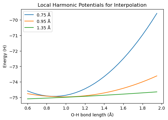
Let’s construct the harmonic potentials based on the three data points we calculated previously. To plot the results let’s use an array of new O-H bond distances.
distlist = np.arange(0.6, 2.0, 0.05)

# list of harmonic potentials
harmonic_potentials = []

for i in range(n_data_pts):
    q_a = qs[i]
    e_a = energies[i]
    g_a = int_gradients[i]
    h_a = int_hessians[i]

    potential = []

    for oh in distlist:
        # print("Calculating the harmonic potential for... ", oh)

        # Create new molecule
        mol_str = mol_template.replace("OHdist", str(oh))
        new_molecule = vlx.Molecule.read_molecule_string(mol_str, units="angstrom")
        cart_coords = new_molecule.get_coordinates_in_bohr()
        q = get_internal_coordinates_array(internal_coordinates, cart_coords)

        # Calculate harmonic potential at point q
        pot = get_harmonic_potential(q_a, e_a, g_a, h_a, q)
        potential.append(pot)
    harmonic_potentials.append(np.array(potential))
Let’s plot the results.
plt.figure(figsize=(6, 4))
plt.title("Local Harmonic Potentials for Interpolation")
plt.plot(distlist, harmonic_potentials[0], label="0.75 Å")
plt.plot(distlist, harmonic_potentials[1], label="0.95 Å")
plt.plot(distlist, harmonic_potentials[2], label="1.35 Å")

plt.xlabel("O-H bond length (Å)")
plt.ylabel("Energy (H)")

plt.legend()
plt.show()
Show code cell output
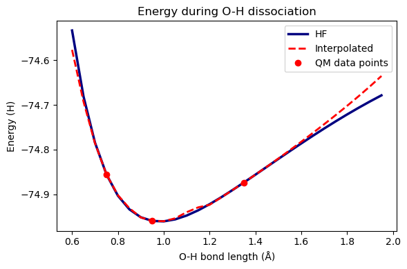
Let’s use these for interpolation and compare to the PES calculated with HF. We need to implement the following equations:
def get_interpolated_pes(
    new_point, data_points, energies, gradients, hessians, exponent
):
    # sum of all interpolation weights -- to normalize them
    sum_weights = 0
    weights = []
    potentials = []

    n_points = len(data_points)

    for i in range(n_points):
        q_a = data_points[i]
        e_a = energies[i]
        g_a = gradients[i]
        h_a = hessians[i]
        dist = np.linalg.norm(new_point - q_a)
        weight = 1 / dist**exponent
        pot = get_harmonic_potential(q_a, e_a, g_a, h_a, new_point)
        # print(pot)
        sum_weights += weight
        weights.append(weight)
        potentials.append(pot)

    new_energy = 0
    for i in range(len(data_points)):
        new_energy += weights[i] / sum_weights * potentials[i]
        # print(en)

    return new_energy
Let’s see how well the interpolated energies compare to HF energies.
scf_energies = []
im_energies = []

for oh in distlist:

    # Create new molecule
    mol_str = mol_template.replace("OHdist", str(oh))
    new_molecule = vlx.Molecule.read_molecule_string(mol_str, units="angstrom")

    # set-up an xtb driver, gradient driver and hessian driver
    new_scf_drv = vlx.ScfRestrictedDriver()
    new_scf_drv.ostream.state = False
    new_scf_results = new_scf_drv.compute(new_molecule, basis)

    # save the results:
    energy = new_scf_drv.get_scf_energy()

    scf_energies.append(energy)

    # calculate energies by interpolation
    coords = new_molecule.get_coordinates_in_bohr()
    new_q = get_internal_coordinates_array(internal_coordinates, coords)
    im_energy = get_interpolated_pes(
        new_q, qs, energies, int_gradients, int_hessians, 12
    )

    im_energies.append(im_energy)
qm_points = [0.75, 0.95, 1.35]

plt.figure(figsize=(6, 4))
plt.title("Energy during O-H dissociation")
plt.plot(distlist, scf_energies, label="HF", linewidth=2.5, color="navy")
plt.plot(distlist, im_energies, "--", label="Interpolated", linewidth=2, color="red")
plt.plot(qm_points, energies, "o", label="QM data points", color="red")

plt.xlabel("O-H bond length (Å)")
plt.ylabel("Energy (H)")

plt.legend()
plt.tight_layout()
plt.show()
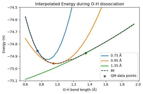
plt.figure(figsize=(6, 4))
plt.title("Interpolated Energy during O-H dissociation")
plt.plot(distlist, harmonic_potentials[0], label="0.75 Å", linewidth=2)
plt.plot(distlist, harmonic_potentials[1], label="0.95 Å", linewidth=2)
plt.plot(distlist, harmonic_potentials[2], label="1.35 Å", linewidth=2)
plt.plot(distlist, im_energies, label="IM", ls="--", color="black")

#plt.plot(qm_points, energies, "o", label="QM data points", color="dimgrey")

plt.scatter(qm_points, energies, label="QM data points", color="dimgrey")
plt.scatter(qm_points[0], energies[0])
plt.scatter(qm_points[1], energies[1])
plt.scatter(qm_points[2], energies[2])

plt.axis(ymin=-75.1, ymax=-74.5)

plt.xlabel("O-H bond length (Å)")
plt.ylabel("Energy (H)")

plt.legend()
plt.tight_layout()
plt.show()
Show code cell output
Things to consider in this approach include:
What happens if you calculate the energy of a configuration which is outside the range of QM data points (eg. an OH bond length larger than the largest value you included)?
What happens if you include more or fewer data points in your data base?