Transition state#
Once we have a suitable candidate for transition state we can optimize the structure for a transition state. As explained before the transition state will be characterized by a vanishing gradient and one negative Hessian
eigenvalue. Therefore, in essence, we are exploring the PES looking for a maximum.
To ilustrate the concepts we will use a simple example in which we will perform the Intrinsic Reaction Coordinate (IRC) method. So, we will start with a transition state candidate and optimize it to transition state. Then we will just minimize the energy in the backward path and the forward path to obtain the reactant and the product as illustrated in the following figure:
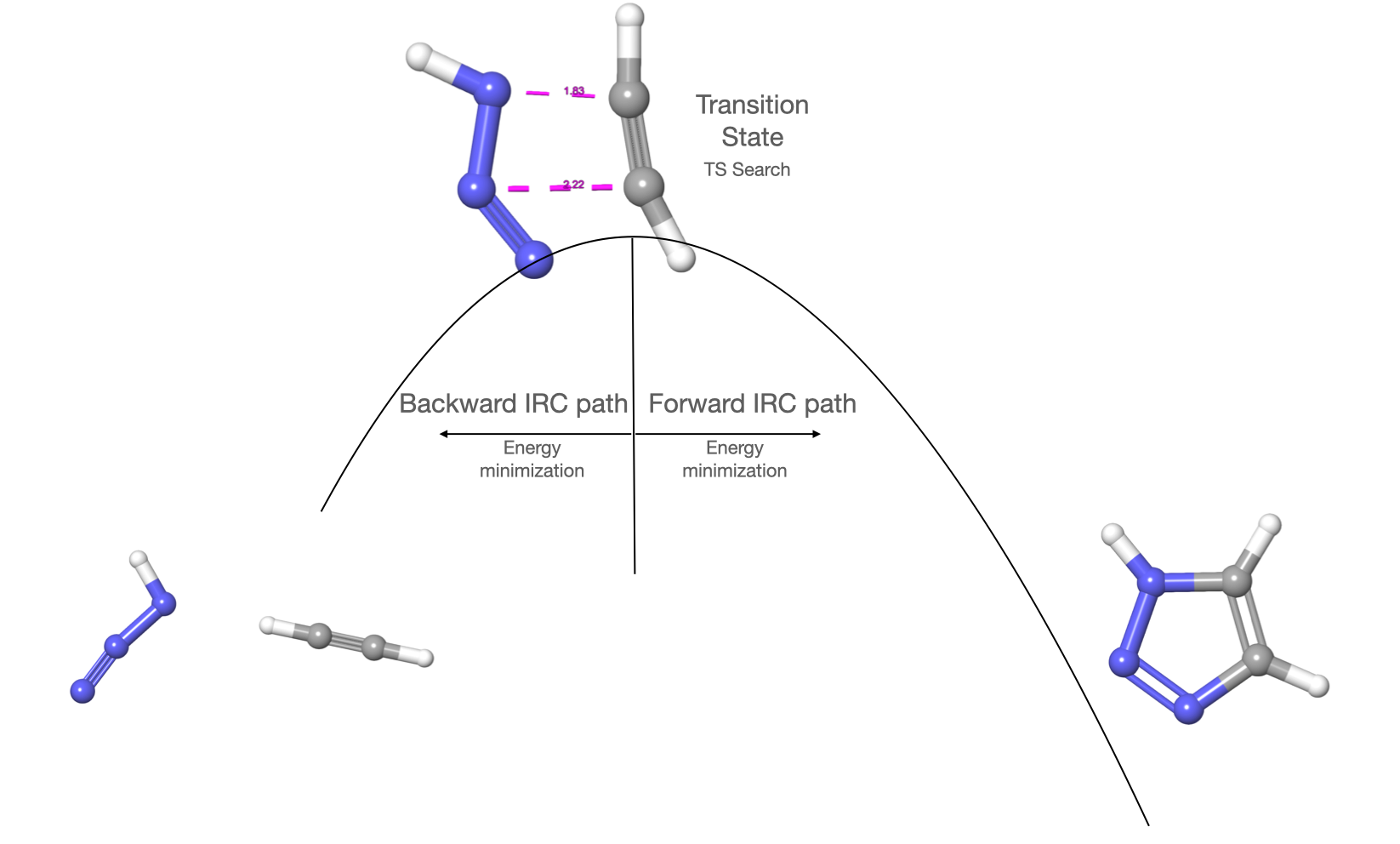
IRC method#
Importing modules#
import veloxchem as vlx
import py3Dmol as p3d
Visualization of the molecule#
First we create a funtion to visualize xyz coordinates and another to compare the geometries
#Function to plot geometries
def drawXYZGeom(geom):
    view = p3d.view(width=400, height=400)
    view.addModel(geom, "xyz")
    view.setStyle({'stick':{}})
    view.zoomTo()
    return(view.show())
## Function to compare geometries
def compXYZGeom(init,final):
    view = p3d.view(linked=True, viewergrid=(1,2),width=400, height=400)
    view.addModel(init, "xyz", viewer = (0,0))
    view.addModel(final, "xyz", viewer = (0,1))
    view.setStyle({'stick':{}})
    view.zoomTo()
    return(view.show())
Then we just introduce the xyz coordinates as a string and we can plot the structure
#Visualizing the structure
geom_xyz = '''8
Initial geometry
C        1.4059000000    0.8128000000    0.0009000000
C        1.5654000000   -0.3926000000    0.0009000000
N       -1.0383000000    1.0196000000   -0.0052000000
H       -2.0386000000    1.4291000000    0.0210000000
H        1.3741000000    1.8940000000   -0.0007000000
H        1.9546000000   -1.4028000000    0.0003000000
N       -0.4958000000   -1.3375000000   -0.0011000000
N       -1.1970000000   -0.3166000000    0.0018000000
'''
drawXYZGeom(geom_xyz)
3Dmol.js failed to load for some reason. Please check your browser console for error messages.
Fig 1: TS candidate
Finding the Transition State#
Setting up the SCF driver#
geometry = vlx.Molecule.read_xyz_string(geom_xyz)
basis = vlx.MolecularBasis.read(geometry,"sto-3g")

scf_drv = vlx.ScfRestrictedDriver()
scf_drv.conv_thresh = 1.0e-10
scf_drv.xcfun = "b3lyp"
scf_drv.grid_level = 4
scf_results = scf_drv.compute(geometry,basis)
Setting up the gradient driver#
scf_grad_drv = vlx.ScfGradientDriver()
scf_grad_drv.compute(geometry,basis,scf_drv)
Setting up the optimization driver#
scf_opt_drv = vlx.OptimizationDriver(scf_grad_drv)
scf_opt_drv.transition = True #We set the option to find transition states
scf_opt_drv.hessian = 'first+last'
scf_opt_drv.compute(geometry,basis,scf_drv)
The output will give four files:
Geometries during the optimization in xyz format (_optim.xyz)
8
Iteration 0 Energy -237.48406869
C        1.4059000000    0.8128000000    0.0009000000
C        1.5654000000   -0.3926000000    0.0009000000
N       -1.0383000000    1.0196000000   -0.0052000000
H       -2.0386000000    1.4291000000    0.0210000000
H        1.3741000000    1.8940000000   -0.0007000000
H        1.9546000000   -1.4028000000    0.0003000000
N       -0.4958000000   -1.3375000000   -0.0011000000
N       -1.1970000000   -0.3166000000    0.0018000000
8
Iteration 1 Energy -237.48588381
C        1.3986767507    0.8076140878    0.0009002477
C        1.5554932198   -0.3912703043    0.0008560542
N       -1.0339417937    1.0131015966   -0.0050309571
H       -2.0296875775    1.4272388306    0.0208045784
H        1.3724942305    1.8878930527   -0.0007271680
H        1.9523159399   -1.3970927549    0.0002038018
N       -0.4855076024   -1.3246755992   -0.0010344286
N       -1.1995439420   -0.3168060274    0.0019270504
8
Iteration 2 Energy -237.48754838
C        1.3881987993    0.8008460851    0.0008959673
C        1.5414491982   -0.3899861931    0.0007853320
N       -1.0276095642    1.0039979473   -0.0047832956
H       -2.0164700299    1.4244073465    0.0205164352
H        1.3697024299    1.8795054853   -0.0007658631
H        1.9489162104   -1.3892473489    0.0000581691
N       -0.4711152364   -1.3064025713   -0.0009230192
N       -1.2027737500   -0.3171424570    0.0021141842
8
.
.
.
Iteration 8 Energy -237.48730935
C        1.2694737152    0.8199118237    0.0020300631
C        1.4650268055   -0.3557331487   -0.0014081365
N       -0.9624886689    0.9369706825   -0.0070753368
H       -1.9114607569    1.3882275308    0.0242133169
H        1.2776270348    1.8879026382    0.0037766854
H        1.9579288423   -1.3019609852   -0.0042985096
N       -0.3994930133   -1.3005046839   -0.0013522025
N       -1.1661868246   -0.3716732596    0.0018726559
8
Iteration 9 Energy -237.48730981
C        1.2687990140    0.8198482259    0.0024123532
C        1.4652286829   -0.3556615967   -0.0016439073
N       -0.9625706742    0.9373517016   -0.0080640143
H       -1.9119100993    1.3873539839    0.0265832651
H        1.2768799142    1.8879461569    0.0046771752
H        1.9591653948   -1.3012461760   -0.0048335460
N       -0.3997144523   -1.3008164821   -0.0025853684
N       -1.1654403884   -0.3717101556    0.0012082555
A log file with the output from Geometric
The initial and final hessian with the Gibbs free energy
The last will look like this:
# == Summary of harmonic free energy analysis ==
# Note: Rotational symmetry is set to 1 regardless of true symmetry
# Note: Free energy does not include contribution from 2 imaginary mode(s)
#
# Gibbs free energy contributions calculated at @ 300.00 K:
# Zero-point vibrational energy:                                   35.1393 kcal/mol
# H   (Trans + Rot + Vib = Tot):   1.4904 +   0.8942 +   0.9940 =   3.3787 kcal/mol
# S   (Trans + Rot + Vib = Tot):  38.6717 +  24.9750 +   4.9343 =  68.5810 cal/mol/K
# TS  (Trans + Rot + Vib = Tot):  11.6015 +   7.4925 +   1.4803 =  20.5743 kcal/mol
#
# Ground State Electronic Energy    : E0                        =  -237.48730981 au (   -149025.5369 kcal/mol)
# Free Energy Correction (Harmonic) : ZPVE + [H-TS]_T,R,V       =     0.02859519 au (        17.9438 kcal/mol)
# Gibbs Free Energy (Harmonic)      : E0 + ZPVE + [H-TS]_T,R,V  =  -237.45871462 au (   -149007.5931 kcal/mol)
#

8
Iteration 9 Energy -237.48730981 (Optimized Structure)
 C    1.2687990140    0.8198482259    0.0024123532
 C    1.4652286829   -0.3556615967   -0.0016439073
 N   -0.9625706742    0.9373517016   -0.0080640143
 H   -1.9119100993    1.3873539839    0.0265832651
 H    1.2768799142    1.8879461569    0.0046771752
 H    1.9591653948   -1.3012461760   -0.0048335460
 N   -0.3997144523   -1.3008164821   -0.0025853684
 N   -1.1654403884   -0.3717101556    0.0012082555
#Comparision initial and final structure
final = '''8
Iteration 9 Energy -237.48730981
C        1.2687990140    0.8198482259    0.0024123532
C        1.4652286829   -0.3556615967   -0.0016439073
N       -0.9625706742    0.9373517016   -0.0080640143
H       -1.9119100993    1.3873539839    0.0265832651
H        1.2768799142    1.8879461569    0.0046771752
H        1.9591653948   -1.3012461760   -0.0048335460
N       -0.3997144523   -1.3008164821   -0.0025853684
N       -1.1654403884   -0.3717101556    0.0012082555
'''
compXYZGeom(geom_xyz,final)
3Dmol.js failed to load for some reason. Please check your browser console for error messages.
Fig 2: : Left side the TS candidate, right side the optimized TS
Visualization of the TS frequencies#
Since the file vdata_lastalso include the displacements for the TS frequency:
 -628.204633
 0.330398  0.000411 -0.001108
 0.368626  0.108966  0.000569
-0.307556  0.056006  0.004238
-0.506299 -0.335269 -0.039828
-0.199547 -0.012314  0.001551
-0.295694 -0.218857 -0.000577
-0.278836 -0.133604  0.000508
 0.059067  0.024571 -0.001489
We can just add the displacements to the TS geometry.
ts = vlx.Molecule.read_xyz_string(final)
coord_ts = ts.get_coordinates()
freq_xyz = '''8
 -628.204633 cm-1
C    0.330398  0.000411 -0.001108
C    0.368626  0.108966  0.000569
N   -0.307556  0.056006  0.004238
H   -0.506299 -0.335269 -0.039828
H   -0.199547 -0.012314  0.001551
H   -0.295694 -0.218857 -0.000577
N   -0.278836 -0.133604  0.000508
N    0.059067  0.024571 -0.001489
'''
freq = vlx.Molecule.read_xyz_string(freq_xyz)
coord_freq = freq.get_coordinates()
vibrations = coord_ts + coord_freq
Now we can just represent the TS creating a xyz file with the initial and final coordinates
ts_vib = '''8
Vibrations on the TS
C        1.2687990140    0.8198482259    0.0024123532   3.02204438e+00  1.55006529e+00  2.46487032e-03
C        1.4652286829   -0.3556615967   -0.0016439073   3.46548310e+00 -4.66187114e-01 -2.03128041e-03
N       -0.9625706742    0.9373517016   -0.0080640143  -2.40019156e+00  1.87717400e+00 -7.23011918e-03
H       -1.9119100993    1.3873539839    0.0265832651  -4.56975291e+00  1.98815248e+00 -2.50289216e-02
H        1.2768799142    1.8879461569    0.0046771752   2.03586415e+00  3.54443109e+00  1.17695454e-02
H        1.9591653948   -1.3012461760   -0.0048335460   3.14350535e+00 -2.87257868e+00 -1.02244501e-02
N       -0.3997144523   -1.3008164821   -0.0025853684  -1.28227452e+00 -2.71066186e+00 -3.92565734e-03
N       -1.1654403884   -0.3717101556    0.0012082555  -2.09074270e+00 -6.55997931e-01 -5.30530216e-04
'''
print("This is the TS freq at -628.20 cm-1.")
view = p3d.view(width=300, height=300)
view.addModel(ts_vib, "xyz", {'vibrate': {'frames':10,'amplitude':0.1}})
view.setStyle({'stick':{}})
view.animate({'loop': 'backAndForth'})
view.zoomTo()
view.show()
This is the TS freq at -628.20 cm-1.
3Dmol.js failed to load for some reason. Please check your browser console for error messages.
Fig 3: Animation of the TS
Calculation of the activation free energy#
By definition the activation free energy is \(\Delta G^{\ddagger} = G^{\ddagger} - G_{react}\). So we just need to get the free energy of the reactant. Since we have observed that the candidate to TS that we have optimized before is further away than the TS (backwards in the IRC path), minimizing that structure will lead to the reactant.
## Going to reactant by minimizing the structure
scf_opt_drv = vlx.OptimizationDriver(scf_grad_drv)
scf_opt_drv.transition = False ## Will only minimize the energy, value by default
scf_opt_drv.hessian = 'last'
scf_opt_drv.compute(geometry,basis,scf_drv)
Comparing reactant and transition state#
reactant = '''8
Iteration 42 Energy -237.52638154 (Optimized Structure)
 C    1.9112351040    0.1624677572   -0.0006980640
 C    3.0548281772   -0.0782577796    0.0004981290
 N   -1.3015267488    0.8281271773    0.0008357891
 H   -1.8259069457    1.7432222546    0.0231535592
 H    0.8632242900    0.3826709271   -0.0017612332
 H    4.0964503076   -0.2975291731    0.0015528206
 N   -2.9848455585   -0.9798798745   -0.0056716903
 N   -2.2831586608   -0.0548212877   -0.0000093104
'''
compXYZGeom(final,reactant)
3Dmol.js failed to load for some reason. Please check your browser console for error messages.
Fig 4: Left side the TS , right side the optimized reactant
Indeed, we can see how see that in the reactant the molecules are further away.
From the outputs of the TS and reactant we can get the activation free energy \(\Delta G^{\ddagger}\) that we can relate with TST to estimate the rate of the reaction.
From the vdata_last files we can get the free energy:
Gibbs Free Energy TS (Harmonic)      : E0 + ZPVE + [H-TS]_T,R,V  =  -237.45871462 au (   -149007.5931 kcal/mol)
Gibbs Free Energy Reactant (Harmonic)      : E0 + ZPVE + [H-TS]_T,R,V  =  -237.50434988 au (   -149036.2297 kcal/mol)
So, the activation free energy will be \(\Delta G^{\ddagger} = G^{\ddagger} - G_{react}\)
g_ts = -149007.5931
g_reac = -149036.2297
delta_g = g_ts-g_reac
print('Activation Free Energy in kcal/mol is:',"%.2f" % delta_g)
Activation Free Energy in kcal/mol is: 28.64
Applying Transition State Theory we can estimate the rate with the Eyring equation:
\( k = \frac{k_B T}{h}\exp(\frac{-\Delta G^{\ddagger}}{RT}) \)
\(R\) in kcal/mol K is 1.958e-3
\(T\) is 300 K
\(k_B\) in J/K is 1.3806e-23
\(h\) in J s is 6.6261e-34
import numpy as np
def rate(delta_g):
    k = (1.3806e-23*300/6.6261e-34)* np.exp(-delta_g/(1.958e-3*300))
    return k
print('The reaction rate is',"%10.3e" % rate(delta_g),'s-1')
The reaction rate is 4.202e-09 s-1
Finding the product#
We will start from a geometry slightly forward in the IRC path from the transition state:
irc_forw_xyz = '''8
Product
C          1.26880        0.81980        0.00240
C          1.46520       -0.35570       -0.00160
N         -0.55580        0.91590       -0.00620
H         -1.50510        1.36590        0.02850
H          1.27690        1.88790        0.00470
H          1.95920       -1.30120       -0.00480
N          0.00710       -1.32220       -0.00070
N         -0.75870       -0.39310        0.00310
'''
drawXYZGeom(irc_forw_xyz)
3Dmol.js failed to load for some reason. Please check your browser console for error messages.
Fig 5: Geometry slightly forward in the IRC that will be used for minimization to product
Note: The bond showed is just a representation artifact.
Minimizing the structure to product: going forward the IRC path#
#SCF driver
geometry = vlx.Molecule.read_xyz_string(prod_xyz)
basis = vlx.MolecularBasis.read(geometry,"sto-3g")

scf_drv = vlx.ScfRestrictedDriver()
scf_drv.conv_thresh = 1.0e-10
scf_drv.xcfun = "b3lyp"
scf_drv.grid_level = 4
scf_results = scf_drv.compute(geometry,basis)

#Gradient driver
scf_grad_drv = vlx.ScfGradientDriver()
scf_grad_drv.compute(geometry,basis,scf_drv)

#Optimization driver
scf_opt_drv = vlx.OptimizationDriver(scf_grad_drv)
scf_opt_drv.transition = False # Option by default
scf_opt_drv.hessian = 'last' #We just need the free energy of the converged geometry
scf_opt_drv.compute(geometry,basis,scf_drv)
The optimized structure shows the pentacycle that we were aiming for
prod_xyz = '''8
Iteration 20 Energy -237.72239707 (Optimized Structure)
 C    0.8617419369    0.8032549747    0.0043906460
 C    1.2297358489   -0.4963316637   -0.0026018408
 N   -0.5141177188    0.7772456796    0.0085738694
 H   -1.1667292050    1.5672508556    0.0149134240
 H    1.4243082245    1.7254211048    0.0060026334
 H    2.2182366655   -0.9261003405   -0.0078164842
 N    0.0829962370   -1.3043435852   -0.0024523167
 N   -0.9785719893   -0.5290970262    0.0043900689
'''
drawXYZGeom(prod_xyz)
3Dmol.js failed to load for some reason. Please check your browser console for error messages.
Fig 6: Geometry of the final geometry
Finally we can determine the reaction free energy \( \Delta G^0 \) as the free energy difference between reactant and product:
As usual we have that data accessible in the vdata_last file:
# == Summary of harmonic free energy analysis ==
# Note: Rotational symmetry is set to 1 regardless of true symmetry
#
# Gibbs free energy contributions calculated at @ 300.00 K:
# Zero-point vibrational energy:                                   41.9789 kcal/mol
# H   (Trans + Rot + Vib = Tot):   1.4904 +   0.8942 +   0.4011 =   2.7857 kcal/mol
# S   (Trans + Rot + Vib = Tot):  38.6717 +  24.0801 +   1.7246 =  64.4763 cal/mol/K
# TS  (Trans + Rot + Vib = Tot):  11.6015 +   7.2240 +   0.5174 =  19.3429 kcal/mol
#
# Ground State Electronic Energy    : E0                        =  -237.72239707 au (   -149173.0564 kcal/mol)
# Free Energy Correction (Harmonic) : ZPVE + [H-TS]_T,R,V       =     0.04051209 au (        25.4217 kcal/mol)
# Gibbs Free Energy (Harmonic)      : E0 + ZPVE + [H-TS]_T,R,V  =  -237.68188498 au (   -149147.6346 kcal/mol)
So, we can just compute the difference:
g_reac = -149036.2297
g_prod = -149147.6346
reac_g = - g_reac + g_prod
print('Reaction Free Energy in kcal/mol is:',"%.2f" % reac_g)
Reaction Free Energy in kcal/mol is: -111.40
With all that information we have profiled the reaction energetics