Cheat sheet

Here we provide quick reference calculation for some of the most common X-ray spectrum calculations, considering XPS/IE, XAS, and (non-resonant) XES of water, as well as a typical workflow.

Typical workflow

• Perform structure optimization

• Calculate the spectra/ionization energies

  • Choose suitable level of theory

  • Depending on spectroscopy:

    • Ionization energy: using \(\Delta\)-methods, or target transitions to extremely diffuse MOs

    • XAS: CVS-ADC, CPP-DFT, or CVS-TDSCF

    • XES: ADC, TDSCF, and using ground state MOs

    • RIXS: two-step model with ADC

• Analysis and assignment of the spectra

  • Looking at amplitudes

  • Visualization

    • Molecular orbitals

    • Natural transition orbitals

    • Attachment/detachment densities

IEs and XPS

Koopmans’ theorem

While it is not recommended for any production calculations, estimates of ionization energies can be obtained from Koopmans’ theorem:

import numpy as np
import veloxchem as vlx

# for vlx
silent_ostream = vlx.OutputStream(None)
from mpi4py import MPI

comm = MPI.COMM_WORLD
# au to eV conversion factor
au2ev = 27.211386

water_mol_str = """
O       0.0000000000     0.0000000000     0.1178336003
H      -0.7595754146    -0.0000000000    -0.4713344012
H       0.7595754146     0.0000000000    -0.4713344012
"""

# Create veloxchem mol and basis objects
mol_vlx = vlx.Molecule.read_molecule_string(water_mol_str)
bas_vlx = vlx.MolecularBasis.read(mol_vlx, "6-31G")

# Perform SCF calculation
scf_gs = vlx.ScfRestrictedDriver(comm, ostream=silent_ostream)
scf_results = scf_gs.compute(mol_vlx, bas_vlx)

# Extract orbital energies
orbital_energies = scf_results["E_alpha"]

print("1s E from Koopmans' theorem:", np.around(au2ev * orbital_energies[0], 2), "eV")

1s E from Koopmans' theorem: -559.5 eV

\(\Delta\)-methods

Substantially improved ionization energies are obtained using \(\Delta\)-methods, where the energy difference of the ground state and core-hole state is used to estimate the IE:

Note

pyscf version - to be changed

import copy

import numpy as np
from pyscf import gto, mp, scf

water_xyz = """
O       0.0000000000     0.0000000000     0.1178336003
H      -0.7595754146    -0.0000000000    -0.4713344012
H       0.7595754146     0.0000000000    -0.4713344012
"""

# Create pyscf mol object
mol = gto.Mole()
mol.atom = water_xyz
mol.basis = "6-31G"
mol.build()

# Perform unrestricted SCF calculation
scf_gs = scf.UHF(mol)
scf_gs.kernel()

# Copy molecular orbitals and occupations
mo0 = copy.deepcopy(scf_gs.mo_coeff)
occ0 = copy.deepcopy(scf_gs.mo_occ)

# Create 1s core-hole by setting alpha_0 population to zero
occ0[0][0] = 0.0

# Perform unrestricted SCF calculation with MOM constraint
scf_ion = scf.UHF(mol)
scf.addons.mom_occ(scf_ion, mo0, occ0)
scf_ion.kernel()

# Run MP2 on neutral and core-hole state
mp_res = mp.MP2(scf_gs).run()
mp_ion = mp.MP2(scf_ion).run()

# IE from energy difference
print(
    "HF ionization energy:",
    np.around(au2ev * (scf_ion.energy_tot() - scf_gs.energy_tot()), 2),
    "eV",
)
print(
    "MP2 ionzation energy:", np.around(au2ev * (mp_ion.e_tot - mp_res.e_tot), 2), "eV"
)

XAS

CVS-ADC

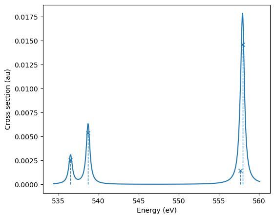
Absorption spectra can be calculated using CVS-ADC:

import gator
import matplotlib.pyplot as plt

water_mol_str = """
O       0.0000000000     0.0000000000     0.1178336003
H      -0.7595754146    -0.0000000000    -0.4713344012
H       0.7595754146     0.0000000000    -0.4713344012
"""

# Construct structure and basis objects
struct = gator.get_molecule(water_mol_str)
basis = gator.get_molecular_basis(struct, "6-31G")

# Perform SCF calculation
scf_gs = gator.run_scf(struct, basis)

# Calculate the 6 lowest eigenstates with CVS restriction to MO #1 (oxygen 1s)
adc_res = gator.run_adc(
    struct, basis, scf_gs, method="cvs-adc2x", singlets=4, core_orbitals=1
)

# Print information on eigenstates
print(adc_res.describe())

plt.figure(figsize=(6, 5))
# Convolute using functionalities available in gator and adcc
adc_res.plot_spectrum()
plt.show()

+--------------------------------------------------------------+
| cvs-adc2x                               singlet ,  converged |
+--------------------------------------------------------------+
|  #        excitation energy     osc str    |v1|^2    |v2|^2  |
|          (au)           (eV)                                 |
|  0      19.71638      536.5099   0.0178       0.8       0.2  |
|  1       19.7967      538.6956   0.0373    0.8087    0.1913  |
|  2      20.49351      557.6567   0.0099    0.7858    0.2142  |
|  3      20.50482      557.9647   0.1016    0.8441    0.1559  |
+--------------------------------------------------------------+

CPP-DFT

• To be added

XES

ADC

The non-resonant X-ray emission spectrum can be calculated with a two-step approach using ADC:

Note

pyscf version - to be changed

import copy

import adcc
import matplotlib.pyplot as plt
import numpy as np
from pyscf import gto, mp, scf

water_xyz = """
O       0.0000000000     0.0000000000     0.1178336003
H      -0.7595754146    -0.0000000000    -0.4713344012
H       0.7595754146     0.0000000000    -0.4713344012
"""

# Create pyscf mol object
mol = gto.Mole()
mol.atom = water_xyz
mol.basis = "6-31G"
mol.build()

# Perform unrestricted SCF calculation
scf_res = scf.UHF(mol)
scf_res.kernel()

# Copy molecular orbitals
mo0 = copy.deepcopy(scf_res.mo_coeff)
occ0 = copy.deepcopy(scf_res.mo_occ)

# Create 1s core-hole by setting alpha_0 population to zero
occ0[0][0] = 0.0

# Perform unrestricted SCF calculation with MOM constraint
scf_ion = scf.UHF(mol)
scf.addons.mom_occ(scf_ion, mo0, occ0)
scf_ion.kernel()

# Perform ADC calculation
adc_xes = adcc.adc2(scf_ion, n_states=4)

# Print information on eigenstates
print(adc_xes.describe())

plt.figure(figsize=(6, 5))
# Convolute using functionalities available in gator and adcc
adc_xes.plot_spectrum()
plt.show()

Ground state MOs

To be added, using the approach here.