Vibrational analysis#
The following steps are carried out mostly by the geomeTRIC module [WS16], hence they are described in less detail. For more details on the topic, the reader is referred to Molecular Vibrations by Wilson, Decius and Cross [WDC80].
Cartesian and mass-weighted Hessian#
The starting point for the vibrational analysis of molecules is the Hessian matrix in Cartesian coordinates, \(\mathbf{H}^{\text{Cart}}\), calculated either numerically or analytically as described in the previous section. Generally, the elements of \(\mathbf{H}^{\text{Cart}}\) are given by second derivatives of the energy \(E\) with respect to nuclear displacement
Hence, \(\mathbf{H}^{\text{Cart}}\) is a \(3N \times 3N\) matrix (where \(N\) is the number of atoms), and \(x_1, x_2, \ldots, x_{3N}\) denote displacements of the Cartesian coordiates. The ‘\(0\)’ subscript indicates that the second deriatives are taken at the equilibrium geometry, where the first derivatives (or gradient) vanish.
As a first step, the Hessian is converted to mass-weighted Cartesian coordinates (MWC), \(\bar{x}_1 = \sqrt{m_1} x_1\), \(\bar{x}_2 = \sqrt{m_1} x_2 \), \(\ldots\), \(\bar{x}_{3N} = \sqrt{m_N} x_{3N}\), where \(m_i\) is the mass of atom \(i\), such that \(\mathbf{H}^{\text{MWC}}\) is given by
Diagonalizing this Hessian gives \(3N\) eigenvalues which represent the fundamental frequencies of the molecule, but include translation and rotational modes.
Translating and rotating frame#
In order to remove translational and rotational degrees of freedom, one first determines the center of mass (COM) \(\mathbf{R}^{\text{COM}}\) in the usual way
where the sum runs over all atoms \(K\), and the origin is then shifted to the COM, \(\mathbf{R}_{K}^{\text{COM}} = \mathbf{R}_K - \mathbf{R}^{\text{COM}}\). Subsequently, one determines the inertia tensor and diagonalizes it to obtain principal moments and axes of inertia. Next, one needs to find the transformation from mass-weighted Cartesian coordinates to a set of \(3N\) coordinates, where the molecule’s translation and rotation are separated out, leaving \(3N - 6\) (or \(3N-5\) for linear molecules) vibrational modes.
This is achieved by applying the so-called Eckart conditions [Eck35]. While the three vectors of length \(3N\) corresponding to translation are simply given by \(\sqrt{m_i}\) times the coordinate axis, the vectors corresponding to rotational motion of the atoms are obtained from the coordinates of the atoms with respect to the COM and the corresponding row of the matrix used to diagonalize the moment of inertia tensor. In the next step, these vectors are normalized and a Gram–Schmidt orthogonalization is carried out to create \(N_\text{vib} = 3N-6\) (or \(3N-5\)) remaining vectors, which are orthogonal to the five or six translational and rotational vectors. Thus, one obtains a transformation matrix \(\mathbf{B}\) which allows for the transformation of the mass-weighted Cartesian coordinates \(\mathbf{\bar{x}}\) to internal coordinates \(\mathbf{\bar{q}} = \mathbf{B\bar{x}}\), where translation and rotation have been projected out.
Hessian in internal coordinates and harmonic frequencies#
Now the Hessian \(\mathbf{H}^\text{MWC}\), which is still given in mass-weighted Cartesian coordinates, is transformed the the internal coordinate system,
yielding a representation in \(N_\text{vib}\) internal coordinates from the full \(3N\) Cartesian coordinates. The Hessian in internal coordinates \(\mathbf{H}^{\text{Int}}\) is successively diagonalized,
where \(\mathbf{\Lambda}\) is the diagonal matrix of \(N_{\text{vib}}\) eigenvalues \(\lambda_i\) which are related to the harmonic vibrational frequencies \(\nu_i\) and \(\mathbf{L}\) is the transformation matrix composed of the eigenvectors.
Finally, the eigenvalues \(\lambda_i = 4 \pi^2 \nu_i^2\) can be converted from frequencies \(\nu_i\) to wavenumbers \(\tilde{\nu}_i\) in reciprocal centimeters by using the relationship \(\nu_i = c \tilde{\nu}_i\), where \(c\) is the speed of light.The wavenumbers are thus obtained from
and successively appropriate conversion factors are applied to obtain the wavenumbers in inverse centimeters (cm\(^{-\text{1}}\)).
Cartesian displacements, reduced masses, and force constants#
The Cartesian normal modes \(\mathbf{l}^{\text{Cart}}\) are obtained by combining this and this equation together with a diagonal matrix \(\mathbf{M}\) defined by \(M_{ii} = \frac{1}{\sqrt{m_i}}\) to undo the mass-weighting, \(\mathbf{l}^{\text{Cart}} = \mathbf{M D L}\), with the individual elements of this matrix being given by
The (normalized) column vectors of \(\mathbf{l}^{\text{Cart}}\) correspond to the normal-mode displacements in Cartesian coordinates, which are used together with property gradients for the calculation of spectral intensities as described here.
From the Cartesian normal modes \(\mathbf{l}^{\text{Cart}}\), the reduced mass \(\mu_i\) of vibration \(i\) can be calculated as
Using the reduced masses, the corresponding force constants \(k_i\) are calculated as
since \(\tilde{\nu}_i = \frac{1}{2 \pi} \sqrt{\frac{k_i}{\mu_i}}\).
The spectral intensities are calculated from the dipole moment gradient (IR spectroscopy), or the polarizability gradient (Raman spectroscopy).
Practical example#
We can perform a vibrational analysis using the VibrationalAnalysis class of VeloxChem. Let us create a molecule, optimize the geometry, and run the vibrational analysis on the optimized geometry.
import veloxchem as vlx
molecule = vlx.Molecule.read_smiles("C=C")
basis = vlx.MolecularBasis.read(molecule, "def2-svp")

scf_drv = vlx.ScfRestrictedDriver()
scf_drv.xcfun = "b3lyp"
scf_results = scf_drv.compute(molecule, basis)
Show code cell output
                                            Self Consistent Field Driver Setup
                                           ====================================

                   Wave Function Model             : Spin-Restricted Kohn-Sham
                   Initial Guess Model             : Superposition of Atomic Densities
                   Convergence Accelerator         : Two Level Direct Inversion of Iterative Subspace
                   Max. Number of Iterations       : 50
                   Max. Number of Error Vectors    : 10
                   Convergence Threshold           : 1.0e-06
                   ERI Screening Threshold         : 1.0e-12
                   Linear Dependence Threshold     : 1.0e-06
                   Exchange-Correlation Functional : B3LYP
                   Molecular Grid Level            : 4

* Info * Nuclear repulsion energy: 33.4144056902 a.u.

* Info * Using the B3LYP functional.

         P. J. Stephens, F. J. Devlin, C. F. Chabalowski, and M. J. Frisch.,  J. Phys. Chem. 98, 11623 (1994)

* Info * Using the Libxc library (v7.0.0).

         S. Lehtola, C. Steigemann, M. J.T. Oliveira, and M. A.L. Marques.,  SoftwareX 7, 1–5 (2018)

* Info * Using the following algorithm for XC numerical integration.

         J. Kussmann, H. Laqua and C. Ochsenfeld, J. Chem. Theory Comput. 2021, 17, 1512-1521
* Info * Molecular grid with 78952 points generated in 0.07 sec.

* Info * Overlap matrix computed in 0.00 sec.

* Info * Kinetic energy matrix computed in 0.00 sec.

* Info * Nuclear potential matrix computed in 0.00 sec.
* Info * Orthogonalization matrix computed in 0.00 sec.
* Info * Starting Reduced Basis SCF calculation...
* Info * ...done. SCF energy in reduced basis set: -77.938548719761 a.u. Time: 0.19 sec.
* Info * Overlap matrix computed in 0.00 sec.

* Info * Kinetic energy matrix computed in 0.00 sec.

* Info * Nuclear potential matrix computed in 0.00 sec.
* Info * Orthogonalization matrix computed in 0.00 sec.
               Iter. |    Kohn-Sham Energy | Energy Change | Gradient Norm | Max. Gradient | Density Change
               --------------------------------------------------------------------------------------------
                  1       -78.527727492841    0.0000000000      0.14831493      0.01830167      0.00000000
2 -78.528058754621 -0.0003312618 0.14304963 0.01840565 0.10324180
3 -78.530924656152 -0.0028659015 0.00108456 0.00017587 0.04603998
4 -78.530924850552 -0.0000001944 0.00016813 0.00002085 0.00060961
5 -78.530924854064 -0.0000000035 0.00003096 0.00000356 0.00006556
6 -78.530924854199 -0.0000000001 0.00000261 0.00000035 0.00001552
7 -78.530924854200 -0.0000000000 0.00000142 0.00000020 0.00000116
8 -78.530924854200 -0.0000000000 0.00000020 0.00000003 0.00000046
*** SCF converged in 8 iterations. Time: 3.01 sec.
               Spin-Restricted Kohn-Sham:
               --------------------------
               Total Energy                       :      -78.5309248542 a.u.
               Electronic Energy                  :     -111.9453305444 a.u.
               Nuclear Repulsion Energy           :       33.4144056902 a.u.
               ------------------------------------
               Gradient Norm                      :        0.0000001972 a.u.


               Ground State Information
               ------------------------
               Charge of Molecule            :  0.0
               Multiplicity (2S+1)           :  1
               Magnetic Quantum Number (M_S) :  0.0


                                                 Spin Restricted Orbitals
                                                 ------------------------

               Molecular Orbital No.   4:
               --------------------------
               Occupation: 2.000 Energy:   -0.57122 a.u.
               (   1 C   1s  :     0.16) (   1 C   2s  :    -0.32) (   2 C   1s  :    -0.16)
               (   2 C   2s  :     0.32) (   3 H   1s  :    -0.19) (   4 H   1s  :    -0.19)
               (   5 H   1s  :     0.19) (   6 H   1s  :     0.19)

               Molecular Orbital No.   5:
               --------------------------
               Occupation: 2.000 Energy:   -0.47382 a.u.
               (   1 C   1p0 :     0.29) (   2 C   1p0 :     0.29) (   3 H   1s  :     0.20)
               (   4 H   1s  :    -0.20) (   5 H   1s  :    -0.20) (   6 H   1s  :     0.20)

               Molecular Orbital No.   6:
               --------------------------
               Occupation: 2.000 Energy:   -0.41619 a.u.
               (   1 C   1p-1:    -0.35) (   1 C   1p0 :     0.17) (   2 C   1p-1:     0.35)
               (   2 C   1p0 :    -0.17) (   3 H   1s  :     0.16) (   4 H   1s  :     0.16)
               (   5 H   1s  :     0.16) (   6 H   1s  :     0.16)

               Molecular Orbital No.   7:
               --------------------------
               Occupation: 2.000 Energy:   -0.35931 a.u.
               (   1 C   1p0 :     0.27) (   2 C   1p0 :    -0.27) (   3 H   1s  :     0.27)
               (   3 H   2s  :     0.16) (   4 H   1s  :    -0.27) (   4 H   2s  :    -0.16)
               (   5 H   1s  :     0.27) (   5 H   2s  :     0.16) (   6 H   1s  :    -0.27)
               (   6 H   2s  :    -0.16)

               Molecular Orbital No.   8:
               --------------------------
               Occupation: 2.000 Energy:   -0.27597 a.u.
               (   1 C   1p+1:    -0.36) (   1 C   1p-1:    -0.18) (   1 C   2p+1:    -0.24)
               (   2 C   1p+1:    -0.36) (   2 C   1p-1:    -0.18) (   2 C   2p+1:    -0.24)

               Molecular Orbital No.   9:
               --------------------------
               Occupation: 0.000 Energy:    0.00649 a.u.
               (   1 C   1p+1:     0.38) (   1 C   1p-1:     0.18) (   1 C   2p+1:     0.57)
               (   1 C   2p-1:     0.28) (   2 C   1p+1:    -0.38) (   2 C   1p-1:    -0.18)
               (   2 C   2p+1:    -0.57) (   2 C   2p-1:    -0.28)

               Molecular Orbital No.  10:
               --------------------------
               Occupation: 0.000 Energy:    0.08177 a.u.
               (   1 C   2s  :     0.19) (   1 C   3s  :     1.42) (   1 C   2p+1:     0.16)
               (   1 C   2p-1:    -0.43) (   1 C   2p0 :     0.21) (   2 C   2s  :     0.19)
               (   2 C   3s  :     1.42) (   2 C   2p+1:    -0.16) (   2 C   2p-1:     0.43)
               (   2 C   2p0 :    -0.21) (   3 H   2s  :    -1.02) (   4 H   2s  :    -1.02)
               (   5 H   2s  :    -1.02) (   6 H   2s  :    -1.02)

               Molecular Orbital No.  11:
               --------------------------
               Occupation: 0.000 Energy:    0.10421 a.u.
               (   1 C   1p0 :     0.24) (   1 C   2p+1:    -0.24) (   1 C   2p-1:     0.21)
               (   1 C   2p0 :     0.62) (   2 C   1p0 :     0.24) (   2 C   2p+1:    -0.24)
               (   2 C   2p-1:     0.21) (   2 C   2p0 :     0.62) (   3 H   2s  :    -1.07)
               (   4 H   2s  :     1.07) (   5 H   2s  :     1.07) (   6 H   2s  :    -1.07)

               Molecular Orbital No.  12:
               --------------------------
               Occupation: 0.000 Energy:    0.11850 a.u.
               (   1 C   2s  :    -0.21) (   1 C   3s  :    -2.14) (   2 C   2s  :     0.21)
               (   2 C   3s  :     2.14) (   3 H   2s  :     1.17) (   4 H   2s  :     1.17)
               (   5 H   2s  :    -1.17) (   6 H   2s  :    -1.17)

               Molecular Orbital No.  13:
               --------------------------
               Occupation: 0.000 Energy:    0.18572 a.u.
               (   1 C   1p0 :    -0.23) (   1 C   2p+1:     0.48) (   1 C   2p-1:    -0.44)
               (   1 C   2p0 :    -1.27) (   2 C   1p0 :     0.23) (   2 C   2p+1:    -0.48)
               (   2 C   2p-1:     0.44) (   2 C   2p0 :     1.27) (   3 H   2s  :     1.54)
               (   4 H   2s  :    -1.54) (   5 H   2s  :     1.54) (   6 H   2s  :    -1.54)
                                                Ground State Dipole Moment
                                               ----------------------------

                                   X   :        -0.000005 a.u.        -0.000013 Debye
                                   Y   :        -0.000002 a.u.        -0.000005 Debye
                                   Z   :        -0.000001 a.u.        -0.000003 Debye
                                 Total :         0.000005 a.u.         0.000014 Debye
opt_drv = vlx.OptimizationDriver(scf_drv)
opt_results = opt_drv.compute(molecule, basis, scf_results)
Show code cell output
                                                Optimization Driver Setup
                                               ===========================

                                     Coordinate System       :    TRIC
                                     Constraints             :    No
                                     Max. Number of Steps    :    300
                                     Transition State        :    No
                                     Hessian                 :    never
* Info * Using geomeTRIC for geometry optimization.

         L.-P. Wang and C.C. Song, J. Chem. Phys. 2016, 144, 214108
* Info * Computing energy and gradient...
                                            Self Consistent Field Driver Setup
                                           ====================================

                   Wave Function Model             : Spin-Restricted Kohn-Sham
                   Initial Guess Model             : Superposition of Atomic Densities
                   Convergence Accelerator         : Two Level Direct Inversion of Iterative Subspace
                   Max. Number of Iterations       : 50
                   Max. Number of Error Vectors    : 10
                   Convergence Threshold           : 1.0e-06
                   ERI Screening Threshold         : 1.0e-12
                   Linear Dependence Threshold     : 1.0e-06
                   Exchange-Correlation Functional : B3LYP
                   Molecular Grid Level            : 4

* Info * Nuclear repulsion energy: 33.4144056902 a.u.

* Info * Using the B3LYP functional.

         P. J. Stephens, F. J. Devlin, C. F. Chabalowski, and M. J. Frisch.,  J. Phys. Chem. 98, 11623 (1994)

* Info * Using the Libxc library (v7.0.0).

         S. Lehtola, C. Steigemann, M. J.T. Oliveira, and M. A.L. Marques.,  SoftwareX 7, 1–5 (2018)

* Info * Using the following algorithm for XC numerical integration.

         J. Kussmann, H. Laqua and C. Ochsenfeld, J. Chem. Theory Comput. 2021, 17, 1512-1521
* Info * Molecular grid with 78952 points generated in 0.08 sec.

* Info * Overlap matrix computed in 0.00 sec.

* Info * Kinetic energy matrix computed in 0.00 sec.

* Info * Nuclear potential matrix computed in 0.00 sec.
* Info * Orthogonalization matrix computed in 0.00 sec.
* Info * Starting Reduced Basis SCF calculation...
* Info * ...done. SCF energy in reduced basis set: -77.938548719761 a.u. Time: 0.19 sec.
* Info * Overlap matrix computed in 0.00 sec.

* Info * Kinetic energy matrix computed in 0.00 sec.

* Info * Nuclear potential matrix computed in 0.00 sec.
* Info * Orthogonalization matrix computed in 0.00 sec.
               Iter. |    Kohn-Sham Energy | Energy Change | Gradient Norm | Max. Gradient | Density Change
               --------------------------------------------------------------------------------------------
                  1       -78.527727492841    0.0000000000      0.14831493      0.01830167      0.00000000
2 -78.528058754621 -0.0003312618 0.14304963 0.01840565 0.10324180
3 -78.530924656152 -0.0028659015 0.00108456 0.00017587 0.04603998
4 -78.530924850552 -0.0000001944 0.00016813 0.00002085 0.00060961
5 -78.530924854064 -0.0000000035 0.00003096 0.00000356 0.00006556
6 -78.530924854199 -0.0000000001 0.00000261 0.00000035 0.00001552
7 -78.530924854200 -0.0000000000 0.00000142 0.00000020 0.00000116
8 -78.530924854200 -0.0000000000 0.00000020 0.00000003 0.00000046
* Info * Checkpoint written to file: vlx_20250709_d6645e4f_scf.h5

               *** SCF converged in 8 iterations. Time: 3.26 sec.
               Spin-Restricted Kohn-Sham:
               --------------------------
               Total Energy                       :      -78.5309248542 a.u.
               Electronic Energy                  :     -111.9453305444 a.u.
               Nuclear Repulsion Energy           :       33.4144056902 a.u.
               ------------------------------------
               Gradient Norm                      :        0.0000001972 a.u.


               Ground State Information
               ------------------------
               Charge of Molecule            :  0.0
               Multiplicity (2S+1)           :  1
               Magnetic Quantum Number (M_S) :  0.0


                                                 Spin Restricted Orbitals
                                                 ------------------------

               Molecular Orbital No.   4:
               --------------------------
               Occupation: 2.000 Energy:   -0.57122 a.u.
               (   1 C   1s  :     0.16) (   1 C   2s  :    -0.32) (   2 C   1s  :    -0.16)
               (   2 C   2s  :     0.32) (   3 H   1s  :    -0.19) (   4 H   1s  :    -0.19)
               (   5 H   1s  :     0.19) (   6 H   1s  :     0.19)

               Molecular Orbital No.   5:
               --------------------------
               Occupation: 2.000 Energy:   -0.47382 a.u.
               (   1 C   1p0 :     0.29) (   2 C   1p0 :     0.29) (   3 H   1s  :     0.20)
               (   4 H   1s  :    -0.20) (   5 H   1s  :    -0.20) (   6 H   1s  :     0.20)

               Molecular Orbital No.   6:
               --------------------------
               Occupation: 2.000 Energy:   -0.41619 a.u.
               (   1 C   1p-1:    -0.35) (   1 C   1p0 :     0.17) (   2 C   1p-1:     0.35)
               (   2 C   1p0 :    -0.17) (   3 H   1s  :     0.16) (   4 H   1s  :     0.16)
               (   5 H   1s  :     0.16) (   6 H   1s  :     0.16)

               Molecular Orbital No.   7:
               --------------------------
               Occupation: 2.000 Energy:   -0.35931 a.u.
               (   1 C   1p0 :     0.27) (   2 C   1p0 :    -0.27) (   3 H   1s  :     0.27)
               (   3 H   2s  :     0.16) (   4 H   1s  :    -0.27) (   4 H   2s  :    -0.16)
               (   5 H   1s  :     0.27) (   5 H   2s  :     0.16) (   6 H   1s  :    -0.27)
               (   6 H   2s  :    -0.16)

               Molecular Orbital No.   8:
               --------------------------
               Occupation: 2.000 Energy:   -0.27597 a.u.
               (   1 C   1p+1:    -0.36) (   1 C   1p-1:    -0.18) (   1 C   2p+1:    -0.24)
               (   2 C   1p+1:    -0.36) (   2 C   1p-1:    -0.18) (   2 C   2p+1:    -0.24)

               Molecular Orbital No.   9:
               --------------------------
               Occupation: 0.000 Energy:    0.00649 a.u.
               (   1 C   1p+1:     0.38) (   1 C   1p-1:     0.18) (   1 C   2p+1:     0.57)
               (   1 C   2p-1:     0.28) (   2 C   1p+1:    -0.38) (   2 C   1p-1:    -0.18)
               (   2 C   2p+1:    -0.57) (   2 C   2p-1:    -0.28)

               Molecular Orbital No.  10:
               --------------------------
               Occupation: 0.000 Energy:    0.08177 a.u.
               (   1 C   2s  :     0.19) (   1 C   3s  :     1.42) (   1 C   2p+1:     0.16)
               (   1 C   2p-1:    -0.43) (   1 C   2p0 :     0.21) (   2 C   2s  :     0.19)
               (   2 C   3s  :     1.42) (   2 C   2p+1:    -0.16) (   2 C   2p-1:     0.43)
               (   2 C   2p0 :    -0.21) (   3 H   2s  :    -1.02) (   4 H   2s  :    -1.02)
               (   5 H   2s  :    -1.02) (   6 H   2s  :    -1.02)

               Molecular Orbital No.  11:
               --------------------------
               Occupation: 0.000 Energy:    0.10421 a.u.
               (   1 C   1p0 :     0.24) (   1 C   2p+1:    -0.24) (   1 C   2p-1:     0.21)
               (   1 C   2p0 :     0.62) (   2 C   1p0 :     0.24) (   2 C   2p+1:    -0.24)
               (   2 C   2p-1:     0.21) (   2 C   2p0 :     0.62) (   3 H   2s  :    -1.07)
               (   4 H   2s  :     1.07) (   5 H   2s  :     1.07) (   6 H   2s  :    -1.07)

               Molecular Orbital No.  12:
               --------------------------
               Occupation: 0.000 Energy:    0.11850 a.u.
               (   1 C   2s  :    -0.21) (   1 C   3s  :    -2.14) (   2 C   2s  :     0.21)
               (   2 C   3s  :     2.14) (   3 H   2s  :     1.17) (   4 H   2s  :     1.17)
               (   5 H   2s  :    -1.17) (   6 H   2s  :    -1.17)

               Molecular Orbital No.  13:
               --------------------------
               Occupation: 0.000 Energy:    0.18572 a.u.
               (   1 C   1p0 :    -0.23) (   1 C   2p+1:     0.48) (   1 C   2p-1:    -0.44)
               (   1 C   2p0 :    -1.27) (   2 C   1p0 :     0.23) (   2 C   2p+1:    -0.48)
               (   2 C   2p-1:     0.44) (   2 C   2p0 :     1.27) (   3 H   2s  :     1.54)
               (   4 H   2s  :    -1.54) (   5 H   2s  :     1.54) (   6 H   2s  :    -1.54)
                                                Ground State Dipole Moment
                                               ----------------------------

                                   X   :        -0.000005 a.u.        -0.000013 Debye
                                   Y   :        -0.000002 a.u.        -0.000005 Debye
                                   Z   :        -0.000001 a.u.        -0.000003 Debye
                                 Total :         0.000005 a.u.         0.000014 Debye
                                                   SCF Gradient Driver
                                                  =====================
Gradient Type : Analytical
                                              Molecular Geometry (Angstroms)
                                             ================================

                          Atom         Coordinate X          Coordinate Y          Coordinate Z

                           C          -0.705876000000        0.193579000000        1.589895000000
                           C          -1.135081000000        1.324228000000        1.034058000000
                           H          -0.848014000000        0.017989000000        2.651302000000
                           H          -0.211235000000       -0.559452000000        0.985001000000
                           H          -0.992947000000        1.499817000000       -0.027351000000
                           H          -1.629737000000        2.077253000000        1.638947000000
                                            Analytical Gradient (Hartree/Bohr)
                                           ------------------------------------

                          Atom           Gradient X            Gradient Y            Gradient Z

                           C           0.002323949078       -0.006126239875        0.003014155791
                           C          -0.002323057810        0.006126358798       -0.003012883691
                           H          -0.001037016791        0.004658660748       -0.005707098892
                           H          -0.003268248149        0.006681250305        0.000131265935
                           H           0.001037012007       -0.004658404286        0.005706231244
                           H           0.003267362593       -0.006681625586       -0.000131670795
*** Time spent in gradient calculation: 2.10 sec ***
* Info *   Energy   : -78.5309248542 a.u.
* Info *   Gradient : 7.364154e-03 a.u. (RMS)
* Info *              7.439725e-03 a.u. (Max)
* Info *   Time     : 5.71 sec
* Info * Computing energy and gradient...
                                            Self Consistent Field Driver Setup
                                           ====================================

                   Wave Function Model             : Spin-Restricted Kohn-Sham
                   Initial Guess Model             : Restart from Checkpoint
                   Convergence Accelerator         : Direct Inversion of Iterative Subspace
                   Max. Number of Iterations       : 50
                   Max. Number of Error Vectors    : 10
                   Convergence Threshold           : 1.0e-06
                   ERI Screening Threshold         : 1.0e-12
                   Linear Dependence Threshold     : 1.0e-06
                   Exchange-Correlation Functional : B3LYP
                   Molecular Grid Level            : 4

* Info * Nuclear repulsion energy: 33.1651813371 a.u.

* Info * Using the B3LYP functional.

         P. J. Stephens, F. J. Devlin, C. F. Chabalowski, and M. J. Frisch.,  J. Phys. Chem. 98, 11623 (1994)

* Info * Using the Libxc library (v7.0.0).

         S. Lehtola, C. Steigemann, M. J.T. Oliveira, and M. A.L. Marques.,  SoftwareX 7, 1–5 (2018)

* Info * Using the following algorithm for XC numerical integration.

         J. Kussmann, H. Laqua and C. Ochsenfeld, J. Chem. Theory Comput. 2021, 17, 1512-1521
* Info * Molecular grid with 79020 points generated in 0.07 sec.

* Info * Restarting from checkpoint file: vlx_20250709_d6645e4f_scf.h5

* Info * Overlap matrix computed in 0.00 sec.

* Info * Kinetic energy matrix computed in 0.00 sec.

* Info * Nuclear potential matrix computed in 0.00 sec.
* Info * Orthogonalization matrix computed in 0.00 sec.
               Iter. |    Kohn-Sham Energy | Energy Change | Gradient Norm | Max. Gradient | Density Change
               --------------------------------------------------------------------------------------------
                  1       -78.519639114770    0.0000000000      0.06877379      0.01284763      0.00000000
2 -78.531356903006 -0.0117177882 0.01265067 0.00170354 0.02896254
3 -78.531361187884 -0.0000042849 0.01276093 0.00161751 0.01145699
4 -78.531384114576 -0.0000229267 0.00052066 0.00004039 0.00422588
5 -78.531384153095 -0.0000000385 0.00009613 0.00001308 0.00028234
6 -78.531384154448 -0.0000000014 0.00000882 0.00000095 0.00003911
7 -78.531384154460 -0.0000000000 0.00000151 0.00000019 0.00000529
8 -78.531384154460 0.0000000000 0.00000194 0.00000027 0.00000098
9 -78.531384154461 -0.0000000000 0.00000012 0.00000001 0.00000058
* Info * Checkpoint written to file: vlx_20250709_d6645e4f_scf.h5

               *** SCF converged in 9 iterations. Time: 3.05 sec.
               Spin-Restricted Kohn-Sham:
               --------------------------
               Total Energy                       :      -78.5313841545 a.u.
               Electronic Energy                  :     -111.6965654915 a.u.
               Nuclear Repulsion Energy           :       33.1651813371 a.u.
               ------------------------------------
               Gradient Norm                      :        0.0000001159 a.u.


               Ground State Information
               ------------------------
               Charge of Molecule            :  0.0
               Multiplicity (2S+1)           :  1
               Magnetic Quantum Number (M_S) :  0.0


                                                 Spin Restricted Orbitals
                                                 ------------------------

               Molecular Orbital No.   4:
               --------------------------
               Occupation: 2.000 Energy:   -0.57267 a.u.
               (   1 C   1s  :     0.16) (   1 C   2s  :    -0.32) (   2 C   1s  :    -0.16)
               (   2 C   2s  :     0.32) (   3 H   1s  :    -0.19) (   4 H   1s  :    -0.19)
               (   5 H   1s  :     0.19) (   6 H   1s  :     0.19)

               Molecular Orbital No.   5:
               --------------------------
               Occupation: 2.000 Energy:   -0.46646 a.u.
               (   1 C   1p0 :     0.29) (   2 C   1p0 :     0.29) (   3 H   1s  :     0.20)
               (   4 H   1s  :    -0.20) (   5 H   1s  :    -0.20) (   6 H   1s  :     0.20)

               Molecular Orbital No.   6:
               --------------------------
               Occupation: 2.000 Energy:   -0.42144 a.u.
               (   1 C   1p-1:    -0.34) (   1 C   1p0 :     0.19) (   2 C   1p-1:     0.34)
               (   2 C   1p0 :    -0.19) (   3 H   1s  :     0.18) (   5 H   1s  :     0.18)

               Molecular Orbital No.   7:
               --------------------------
               Occupation: 2.000 Energy:   -0.35506 a.u.
               (   1 C   1p0 :     0.26) (   2 C   1p0 :    -0.26) (   3 H   1s  :     0.26)
               (   3 H   2s  :     0.16) (   4 H   1s  :    -0.28) (   4 H   2s  :    -0.17)
               (   5 H   1s  :     0.26) (   5 H   2s  :     0.16) (   6 H   1s  :    -0.28)
               (   6 H   2s  :    -0.17)

               Molecular Orbital No.   8:
               --------------------------
               Occupation: 2.000 Energy:   -0.27541 a.u.
               (   1 C   1p+1:    -0.36) (   1 C   1p-1:    -0.18) (   1 C   2p+1:    -0.24)
               (   2 C   1p+1:    -0.36) (   2 C   1p-1:    -0.18) (   2 C   2p+1:    -0.24)

               Molecular Orbital No.   9:
               --------------------------
               Occupation: 0.000 Energy:    0.00462 a.u.
               (   1 C   1p+1:     0.38) (   1 C   1p-1:     0.18) (   1 C   2p+1:     0.56)
               (   1 C   2p-1:     0.27) (   2 C   1p+1:    -0.38) (   2 C   1p-1:    -0.18)
               (   2 C   2p+1:    -0.56) (   2 C   2p-1:    -0.27)

               Molecular Orbital No.  10:
               --------------------------
               Occupation: 0.000 Energy:    0.08265 a.u.
               (   1 C   2s  :     0.19) (   1 C   3s  :     1.42) (   1 C   2p+1:     0.17)
               (   1 C   2p-1:    -0.44) (   1 C   2p0 :     0.21) (   2 C   2s  :     0.19)
               (   2 C   3s  :     1.42) (   2 C   2p+1:    -0.17) (   2 C   2p-1:     0.44)
               (   2 C   2p0 :    -0.21) (   3 H   2s  :    -1.03) (   4 H   2s  :    -1.03)
               (   5 H   2s  :    -1.03) (   6 H   2s  :    -1.03)

               Molecular Orbital No.  11:
               --------------------------
               Occupation: 0.000 Energy:    0.10201 a.u.
               (   1 C   3s  :     0.22) (   1 C   1p0 :     0.25) (   1 C   2p+1:    -0.22)
               (   1 C   2p-1:     0.18) (   1 C   2p0 :     0.61) (   2 C   3s  :    -0.22)
               (   2 C   1p0 :     0.25) (   2 C   2p+1:    -0.22) (   2 C   2p-1:     0.18)
               (   2 C   2p0 :     0.61) (   3 H   2s  :    -1.17) (   4 H   2s  :     0.91)
               (   5 H   2s  :     1.17) (   6 H   2s  :    -0.91)

               Molecular Orbital No.  12:
               --------------------------
               Occupation: 0.000 Energy:    0.11379 a.u.
               (   1 C   2s  :    -0.21) (   1 C   3s  :    -2.06) (   2 C   2s  :     0.21)
               (   2 C   3s  :     2.06) (   3 H   2s  :     1.00) (   4 H   2s  :     1.26)
               (   5 H   2s  :    -1.00) (   6 H   2s  :    -1.26)

               Molecular Orbital No.  13:
               --------------------------
               Occupation: 0.000 Energy:    0.18438 a.u.
               (   1 C   1p0 :    -0.24) (   1 C   2p+1:     0.47) (   1 C   2p-1:    -0.43)
               (   1 C   2p0 :    -1.24) (   2 C   1p0 :     0.24) (   2 C   2p+1:    -0.47)
               (   2 C   2p-1:     0.43) (   2 C   2p0 :     1.24) (   3 H   2s  :     1.51)
               (   4 H   2s  :    -1.49) (   5 H   2s  :     1.51) (   6 H   2s  :    -1.49)
                                                Ground State Dipole Moment
                                               ----------------------------

                                   X   :         0.000002 a.u.         0.000005 Debye
                                   Y   :         0.000001 a.u.         0.000002 Debye
                                   Z   :         0.000000 a.u.         0.000001 Debye
                                 Total :         0.000002 a.u.         0.000006 Debye
                                                   SCF Gradient Driver
                                                  =====================
                          Gradient Type                   : Analytical
                          Exchange-Correlation Functional : B3LYP
                          Molecular Grid Level            : 4
                                              Molecular Geometry (Angstroms)
                                             ================================

                          Atom         Coordinate X          Coordinate Y          Coordinate Z

                           C          -0.708615335998        0.194594057886        1.600433086373
                           C          -1.132350665696        1.323209242813        1.023517397378
                           H          -0.833751497436       -0.018182740506        2.666689462443
                           H          -0.207928978826       -0.574831284020        1.004503666016
                           H          -1.007212909761        1.535986230727       -0.042738736899
                           H          -1.633030671230        2.092638486560        1.619447150602
                                            Analytical Gradient (Hartree/Bohr)
                                           ------------------------------------

                          Atom           Gradient X            Gradient Y            Gradient Z

                           C          -0.001043535237       -0.001313438802        0.007848490676
                           C           0.001043103767        0.001313159186       -0.007848543960
                           H           0.000821927972       -0.001772066975        0.000172285072
                           H          -0.000517836032        0.001504861154       -0.000990409907
                           H          -0.000821918067        0.001772077896       -0.000172249282
                           H           0.000518257253       -0.001504592539        0.000990427514
*** Time spent in gradient calculation: 1.93 sec ***
* Info *   Energy   : -78.5313841545 a.u.
* Info *   Gradient : 4.891199e-03 a.u. (RMS)
* Info *              8.025764e-03 a.u. (Max)
* Info *   Time     : 5.15 sec
* Info * Computing energy and gradient...
                                            Self Consistent Field Driver Setup
                                           ====================================

                   Wave Function Model             : Spin-Restricted Kohn-Sham
                   Initial Guess Model             : Restart from Checkpoint
                   Convergence Accelerator         : Direct Inversion of Iterative Subspace
                   Max. Number of Iterations       : 50
                   Max. Number of Error Vectors    : 10
                   Convergence Threshold           : 1.0e-06
                   ERI Screening Threshold         : 1.0e-12
                   Linear Dependence Threshold     : 1.0e-06
                   Exchange-Correlation Functional : B3LYP
                   Molecular Grid Level            : 4

* Info * Nuclear repulsion energy: 33.1349699715 a.u.

* Info * Using the B3LYP functional.

         P. J. Stephens, F. J. Devlin, C. F. Chabalowski, and M. J. Frisch.,  J. Phys. Chem. 98, 11623 (1994)

* Info * Using the Libxc library (v7.0.0).

         S. Lehtola, C. Steigemann, M. J.T. Oliveira, and M. A.L. Marques.,  SoftwareX 7, 1–5 (2018)

* Info * Using the following algorithm for XC numerical integration.

         J. Kussmann, H. Laqua and C. Ochsenfeld, J. Chem. Theory Comput. 2021, 17, 1512-1521
* Info * Molecular grid with 79044 points generated in 0.08 sec.

* Info * Restarting from checkpoint file: vlx_20250709_d6645e4f_scf.h5

* Info * Overlap matrix computed in 0.00 sec.

* Info * Kinetic energy matrix computed in 0.00 sec.

* Info * Nuclear potential matrix computed in 0.00 sec.
* Info * Orthogonalization matrix computed in 0.00 sec.
               Iter. |    Kohn-Sham Energy | Energy Change | Gradient Norm | Max. Gradient | Density Change
               --------------------------------------------------------------------------------------------
                  1       -78.528919110943    0.0000000000      0.05480533      0.00901206      0.00000000
2 -78.531531160617 -0.0026120497 0.00413281 0.00037288 0.02152129
3 -78.531533687533 -0.0000025269 0.00209531 0.00026473 0.00379429
4 -78.531534252330 -0.0000005648 0.00088442 0.00011054 0.00098666
5 -78.531534360942 -0.0000001086 0.00008176 0.00000992 0.00031420
6 -78.531534361851 -0.0000000009 0.00000437 0.00000048 0.00003598
7 -78.531534361854 -0.0000000000 0.00000141 0.00000018 0.00000298
8 -78.531534361854 0.0000000000 0.00000114 0.00000016 0.00000072
9 -78.531534361854 -0.0000000000 0.00000005 0.00000001 0.00000034
* Info * Checkpoint written to file: vlx_20250709_d6645e4f_scf.h5

               *** SCF converged in 9 iterations. Time: 3.02 sec.
               Spin-Restricted Kohn-Sham:
               --------------------------
               Total Energy                       :      -78.5315343619 a.u.
               Electronic Energy                  :     -111.6665043334 a.u.
               Nuclear Repulsion Energy           :       33.1349699715 a.u.
               ------------------------------------
               Gradient Norm                      :        0.0000000497 a.u.


               Ground State Information
               ------------------------
               Charge of Molecule            :  0.0
               Multiplicity (2S+1)           :  1
               Magnetic Quantum Number (M_S) :  0.0


                                                 Spin Restricted Orbitals
                                                 ------------------------

               Molecular Orbital No.   4:
               --------------------------
               Occupation: 2.000 Energy:   -0.57156 a.u.
               (   1 C   1s  :     0.16) (   1 C   2s  :    -0.32) (   2 C   1s  :    -0.16)
               (   2 C   2s  :     0.32) (   3 H   1s  :    -0.19) (   4 H   1s  :    -0.19)
               (   5 H   1s  :     0.19) (   6 H   1s  :     0.19)

               Molecular Orbital No.   5:
               --------------------------
               Occupation: 2.000 Energy:   -0.46604 a.u.
               (   1 C   1p0 :     0.29) (   2 C   1p0 :     0.29) (   3 H   1s  :     0.20)
               (   4 H   1s  :    -0.20) (   5 H   1s  :    -0.20) (   6 H   1s  :     0.20)

               Molecular Orbital No.   6:
               --------------------------
               Occupation: 2.000 Energy:   -0.42086 a.u.
               (   1 C   1p-1:    -0.35) (   1 C   1p0 :     0.17) (   2 C   1p-1:     0.35)
               (   2 C   1p0 :    -0.17) (   3 H   1s  :     0.16) (   4 H   1s  :     0.17)
               (   5 H   1s  :     0.16) (   6 H   1s  :     0.17)

               Molecular Orbital No.   7:
               --------------------------
               Occupation: 2.000 Energy:   -0.35471 a.u.
               (   1 C   1p0 :     0.28) (   2 C   1p0 :    -0.28) (   3 H   1s  :     0.27)
               (   3 H   2s  :     0.16) (   4 H   1s  :    -0.26) (   4 H   2s  :    -0.16)
               (   5 H   1s  :     0.27) (   5 H   2s  :     0.16) (   6 H   1s  :    -0.26)
               (   6 H   2s  :    -0.16)

               Molecular Orbital No.   8:
               --------------------------
               Occupation: 2.000 Energy:   -0.27561 a.u.
               (   1 C   1p+1:    -0.36) (   1 C   1p-1:    -0.18) (   1 C   2p+1:    -0.24)
               (   2 C   1p+1:    -0.36) (   2 C   1p-1:    -0.18) (   2 C   2p+1:    -0.24)

               Molecular Orbital No.   9:
               --------------------------
               Occupation: 0.000 Energy:    0.00488 a.u.
               (   1 C   1p+1:     0.38) (   1 C   1p-1:     0.18) (   1 C   2p+1:     0.57)
               (   1 C   2p-1:     0.27) (   2 C   1p+1:    -0.38) (   2 C   1p-1:    -0.18)
               (   2 C   2p+1:    -0.57) (   2 C   2p-1:    -0.27)

               Molecular Orbital No.  10:
               --------------------------
               Occupation: 0.000 Energy:    0.08203 a.u.
               (   1 C   2s  :     0.19) (   1 C   3s  :     1.41) (   1 C   2p+1:     0.17)
               (   1 C   2p-1:    -0.44) (   1 C   2p0 :     0.22) (   2 C   2s  :     0.19)
               (   2 C   3s  :     1.41) (   2 C   2p+1:    -0.17) (   2 C   2p-1:     0.44)
               (   2 C   2p0 :    -0.22) (   3 H   2s  :    -1.02) (   4 H   2s  :    -1.02)
               (   5 H   2s  :    -1.02) (   6 H   2s  :    -1.02)

               Molecular Orbital No.  11:
               --------------------------
               Occupation: 0.000 Energy:    0.10128 a.u.
               (   1 C   1p0 :     0.24) (   1 C   2p+1:    -0.23) (   1 C   2p-1:     0.22)
               (   1 C   2p0 :     0.59) (   2 C   1p0 :     0.24) (   2 C   2p+1:    -0.23)
               (   2 C   2p-1:     0.22) (   2 C   2p0 :     0.59) (   3 H   2s  :    -0.97)
               (   4 H   2s  :     1.10) (   5 H   2s  :     0.97) (   6 H   2s  :    -1.10)

               Molecular Orbital No.  12:
               --------------------------
               Occupation: 0.000 Energy:    0.11308 a.u.
               (   1 C   2s  :    -0.21) (   1 C   3s  :    -2.06) (   2 C   2s  :     0.21)
               (   2 C   3s  :     2.06) (   3 H   2s  :     1.20) (   4 H   2s  :     1.07)
               (   5 H   2s  :    -1.20) (   6 H   2s  :    -1.07)

               Molecular Orbital No.  13:
               --------------------------
               Occupation: 0.000 Energy:    0.18427 a.u.
               (   1 C   1p0 :    -0.24) (   1 C   2p+1:     0.47) (   1 C   2p-1:    -0.43)
               (   1 C   2p0 :    -1.24) (   2 C   1p0 :     0.24) (   2 C   2p+1:    -0.47)
               (   2 C   2p-1:     0.43) (   2 C   2p0 :     1.24) (   3 H   2s  :     1.49)
               (   4 H   2s  :    -1.50) (   5 H   2s  :     1.49) (   6 H   2s  :    -1.50)
                                                Ground State Dipole Moment
                                               ----------------------------

                                   X   :         0.000002 a.u.         0.000006 Debye
                                   Y   :         0.000001 a.u.         0.000003 Debye
                                   Z   :         0.000000 a.u.         0.000001 Debye
                                 Total :         0.000003 a.u.         0.000007 Debye
                                                   SCF Gradient Driver
                                                  =====================
                          Gradient Type                   : Analytical
                          Exchange-Correlation Functional : B3LYP
                          Molecular Grid Level            : 4
                                              Molecular Geometry (Angstroms)
                                             ================================

                          Atom         Coordinate X          Coordinate Y          Coordinate Z

                           C          -0.703810057957        0.190487510276        1.587335008298
                           C          -1.137156346692        1.327315698456        1.036614899560
                           H          -0.836837554216       -0.007945949763        2.658004266509
                           H          -0.199885872746       -0.590130497902        1.001663647060
                           H          -1.004126503041        1.525750123577       -0.034053478379
                           H          -1.641073726973        2.107937110575        1.622287685886
                                            Analytical Gradient (Hartree/Bohr)
                                           ------------------------------------

                          Atom           Gradient X            Gradient Y            Gradient Z

                           C           0.000981874927       -0.001458248163       -0.001284542405
                           C          -0.000982368403        0.001458010419        0.001284152287
                           H          -0.000511375364        0.000441222341        0.001386939656
                           H           0.001274863727       -0.002230552992       -0.000904042405
                           H           0.000511430343       -0.000441234392       -0.001386658853
                           H          -0.001274425707        0.002230802472        0.000904152202
*** Time spent in gradient calculation: 2.22 sec ***
* Info *   Energy   : -78.5315343619 a.u.
* Info *   Gradient : 2.201342e-03 a.u. (RMS)
* Info *              2.723625e-03 a.u. (Max)
* Info *   Time     : 5.41 sec
* Info * Computing energy and gradient...
                                            Self Consistent Field Driver Setup
                                           ====================================

                   Wave Function Model             : Spin-Restricted Kohn-Sham
                   Initial Guess Model             : Restart from Checkpoint
                   Convergence Accelerator         : Direct Inversion of Iterative Subspace
                   Max. Number of Iterations       : 50
                   Max. Number of Error Vectors    : 10
                   Convergence Threshold           : 1.0e-06
                   ERI Screening Threshold         : 1.0e-12
                   Linear Dependence Threshold     : 1.0e-06
                   Exchange-Correlation Functional : B3LYP
                   Molecular Grid Level            : 4

* Info * Nuclear repulsion energy: 33.2113498706 a.u.

* Info * Using the B3LYP functional.

         P. J. Stephens, F. J. Devlin, C. F. Chabalowski, and M. J. Frisch.,  J. Phys. Chem. 98, 11623 (1994)

* Info * Using the Libxc library (v7.0.0).

         S. Lehtola, C. Steigemann, M. J.T. Oliveira, and M. A.L. Marques.,  SoftwareX 7, 1–5 (2018)

* Info * Using the following algorithm for XC numerical integration.

         J. Kussmann, H. Laqua and C. Ochsenfeld, J. Chem. Theory Comput. 2021, 17, 1512-1521
* Info * Molecular grid with 79026 points generated in 0.08 sec.

* Info * Restarting from checkpoint file: vlx_20250709_d6645e4f_scf.h5

* Info * Overlap matrix computed in 0.00 sec.

* Info * Kinetic energy matrix computed in 0.00 sec.

* Info * Nuclear potential matrix computed in 0.00 sec.
* Info * Orthogonalization matrix computed in 0.00 sec.
               Iter. |    Kohn-Sham Energy | Energy Change | Gradient Norm | Max. Gradient | Density Change
               --------------------------------------------------------------------------------------------
                  1       -78.536250077134    0.0000000000      0.02376568      0.00450239      0.00000000
2 -78.531589833871 0.0046602433 0.00569922 0.00079101 0.00798787
3 -78.531589875198 -0.0000000413 0.00611683 0.00079064 0.00471686
4 -78.531595186536 -0.0000053113 0.00016855 0.00002196 0.00194915
5 -78.531595190968 -0.0000000044 0.00002796 0.00000396 0.00007181
6 -78.531595191067 -0.0000000001 0.00000275 0.00000032 0.00001310
7 -78.531595191068 -0.0000000000 0.00000051 0.00000007 0.00000137
* Info * Checkpoint written to file: vlx_20250709_d6645e4f_scf.h5

               *** SCF converged in 7 iterations. Time: 2.30 sec.
               Spin-Restricted Kohn-Sham:
               --------------------------
               Total Energy                       :      -78.5315951911 a.u.
               Electronic Energy                  :     -111.7429450617 a.u.
               Nuclear Repulsion Energy           :       33.2113498706 a.u.
               ------------------------------------
               Gradient Norm                      :        0.0000005056 a.u.


               Ground State Information
               ------------------------
               Charge of Molecule            :  0.0
               Multiplicity (2S+1)           :  1
               Magnetic Quantum Number (M_S) :  0.0


                                                 Spin Restricted Orbitals
                                                 ------------------------

               Molecular Orbital No.   4:
               --------------------------
               Occupation: 2.000 Energy:   -0.57216 a.u.
               (   1 C   1s  :     0.16) (   1 C   2s  :    -0.32) (   2 C   1s  :    -0.16)
               (   2 C   2s  :     0.32) (   3 H   1s  :    -0.19) (   4 H   1s  :    -0.19)
               (   5 H   1s  :     0.19) (   6 H   1s  :     0.19)

               Molecular Orbital No.   5:
               --------------------------
               Occupation: 2.000 Energy:   -0.46692 a.u.
               (   1 C   1p0 :     0.29) (   2 C   1p0 :     0.29) (   3 H   1s  :     0.20)
               (   4 H   1s  :    -0.20) (   5 H   1s  :    -0.20) (   6 H   1s  :     0.20)

               Molecular Orbital No.   6:
               --------------------------
               Occupation: 2.000 Energy:   -0.42136 a.u.
               (   1 C   1p-1:    -0.35) (   1 C   1p0 :     0.17) (   2 C   1p-1:     0.35)
               (   2 C   1p0 :    -0.17) (   3 H   1s  :     0.17) (   4 H   1s  :     0.17)
               (   5 H   1s  :     0.17) (   6 H   1s  :     0.17)

               Molecular Orbital No.   7:
               --------------------------
               Occupation: 2.000 Energy:   -0.35499 a.u.
               (   1 C   1p0 :     0.27) (   2 C   1p0 :    -0.27) (   3 H   1s  :     0.27)
               (   3 H   2s  :     0.16) (   4 H   1s  :    -0.27) (   4 H   2s  :    -0.16)
               (   5 H   1s  :     0.27) (   5 H   2s  :     0.16) (   6 H   1s  :    -0.27)
               (   6 H   2s  :    -0.16)

               Molecular Orbital No.   8:
               --------------------------
               Occupation: 2.000 Energy:   -0.27598 a.u.
               (   1 C   1p+1:    -0.36) (   1 C   1p-1:    -0.18) (   1 C   2p+1:    -0.24)
               (   2 C   1p+1:    -0.36) (   2 C   1p-1:    -0.18) (   2 C   2p+1:    -0.24)

               Molecular Orbital No.   9:
               --------------------------
               Occupation: 0.000 Energy:    0.00545 a.u.
               (   1 C   1p+1:     0.38) (   1 C   1p-1:     0.18) (   1 C   2p+1:     0.57)
               (   1 C   2p-1:     0.27) (   2 C   1p+1:    -0.38) (   2 C   1p-1:    -0.18)
               (   2 C   2p+1:    -0.57) (   2 C   2p-1:    -0.27)

               Molecular Orbital No.  10:
               --------------------------
               Occupation: 0.000 Energy:    0.08255 a.u.
               (   1 C   2s  :     0.19) (   1 C   3s  :     1.42) (   1 C   2p+1:     0.17)
               (   1 C   2p-1:    -0.44) (   1 C   2p0 :     0.22) (   2 C   2s  :     0.19)
               (   2 C   3s  :     1.42) (   2 C   2p+1:    -0.17) (   2 C   2p-1:     0.44)
               (   2 C   2p0 :    -0.22) (   3 H   2s  :    -1.03) (   4 H   2s  :    -1.03)
               (   5 H   2s  :    -1.03) (   6 H   2s  :    -1.03)

               Molecular Orbital No.  11:
               --------------------------
               Occupation: 0.000 Energy:    0.10192 a.u.
               (   1 C   1p0 :     0.24) (   1 C   2p+1:    -0.23) (   1 C   2p-1:     0.21)
               (   1 C   2p0 :     0.60) (   2 C   1p0 :     0.24) (   2 C   2p+1:    -0.23)
               (   2 C   2p-1:     0.21) (   2 C   2p0 :     0.60) (   3 H   2s  :    -1.04)
               (   4 H   2s  :     1.04) (   5 H   2s  :     1.04) (   6 H   2s  :    -1.04)

               Molecular Orbital No.  12:
               --------------------------
               Occupation: 0.000 Energy:    0.11386 a.u.
               (   1 C   2s  :    -0.21) (   1 C   3s  :    -2.07) (   2 C   2s  :     0.21)
               (   2 C   3s  :     2.07) (   3 H   2s  :     1.14) (   4 H   2s  :     1.14)
               (   5 H   2s  :    -1.14) (   6 H   2s  :    -1.14)

               Molecular Orbital No.  13:
               --------------------------
               Occupation: 0.000 Energy:    0.18476 a.u.
               (   1 C   1p0 :    -0.24) (   1 C   2p+1:     0.47) (   1 C   2p-1:    -0.43)
               (   1 C   2p0 :    -1.24) (   2 C   1p0 :     0.24) (   2 C   2p+1:    -0.47)
               (   2 C   2p-1:     0.43) (   2 C   2p0 :     1.24) (   3 H   2s  :     1.50)
               (   4 H   2s  :    -1.50) (   5 H   2s  :     1.50) (   6 H   2s  :    -1.50)
                                                Ground State Dipole Moment
                                               ----------------------------

                                   X   :        -0.000001 a.u.        -0.000002 Debye
                                   Y   :         0.000000 a.u.         0.000001 Debye
                                   Z   :        -0.000000 a.u.        -0.000001 Debye
                                 Total :         0.000001 a.u.         0.000002 Debye
                                                   SCF Gradient Driver
                                                  =====================
                          Gradient Type                   : Analytical
                          Exchange-Correlation Functional : B3LYP
                          Molecular Grid Level            : 4
                                              Molecular Geometry (Angstroms)
                                             ================================

                          Atom         Coordinate X          Coordinate Y          Coordinate Z

                           C          -0.705553109194        0.192795734182        1.590286503705
                           C          -1.135409457172        1.325009221997        1.033664312190
                           H          -0.836264546750       -0.009167454757        2.658155757583
                           H          -0.203705137490       -0.582796800011        1.002943075353
                           H          -1.004698297632        1.526972547267       -0.034204956681
                           H          -1.637259485388        2.100600761231        1.621007312737
                                            Analytical Gradient (Hartree/Bohr)
                                           ------------------------------------

                          Atom           Gradient X            Gradient Y            Gradient Z

                           C          -0.000034034491        0.000069473012        0.000001299320
                           C           0.000034189477       -0.000069479876       -0.000001244420
                           H          -0.000034624707        0.000089767989       -0.000043486156
                           H          -0.000013281601        0.000056261007       -0.000067925137
                           H           0.000034630853       -0.000089731425        0.000043449145
                           H           0.000013120551       -0.000056290642        0.000067907247
*** Time spent in gradient calculation: 1.95 sec ***
* Info *   Energy   : -78.5315951911 a.u.
* Info *   Gradient : 9.145055e-05 a.u. (RMS)
* Info *              1.055851e-04 a.u. (Max)
* Info *   Time     : 4.42 sec
* Info * Computing energy and gradient...
                                            Self Consistent Field Driver Setup
                                           ====================================

                   Wave Function Model             : Spin-Restricted Kohn-Sham
                   Initial Guess Model             : Restart from Checkpoint
                   Convergence Accelerator         : Direct Inversion of Iterative Subspace
                   Max. Number of Iterations       : 50
                   Max. Number of Error Vectors    : 10
                   Convergence Threshold           : 1.0e-06
                   ERI Screening Threshold         : 1.0e-12
                   Linear Dependence Threshold     : 1.0e-06
                   Exchange-Correlation Functional : B3LYP
                   Molecular Grid Level            : 4

* Info * Nuclear repulsion energy: 33.2069337910 a.u.

* Info * Using the B3LYP functional.

         P. J. Stephens, F. J. Devlin, C. F. Chabalowski, and M. J. Frisch.,  J. Phys. Chem. 98, 11623 (1994)

* Info * Using the Libxc library (v7.0.0).

         S. Lehtola, C. Steigemann, M. J.T. Oliveira, and M. A.L. Marques.,  SoftwareX 7, 1–5 (2018)

* Info * Using the following algorithm for XC numerical integration.

         J. Kussmann, H. Laqua and C. Ochsenfeld, J. Chem. Theory Comput. 2021, 17, 1512-1521
* Info * Molecular grid with 79026 points generated in 0.08 sec.

* Info * Restarting from checkpoint file: vlx_20250709_d6645e4f_scf.h5

* Info * Overlap matrix computed in 0.00 sec.

* Info * Kinetic energy matrix computed in 0.00 sec.

* Info * Nuclear potential matrix computed in 0.00 sec.
* Info * Orthogonalization matrix computed in 0.00 sec.
               Iter. |    Kohn-Sham Energy | Energy Change | Gradient Norm | Max. Gradient | Density Change
               --------------------------------------------------------------------------------------------
                  1       -78.531428491684    0.0000000000      0.00106264      0.00022852      0.00000000
2 -78.531595381877 -0.0001668902 0.00024801 0.00003205 0.00043565
3 -78.531595383591 -0.0000000017 0.00023598 0.00002945 0.00020947
4 -78.531595391245 -0.0000000077 0.00001576 0.00000179 0.00007938
5 -78.531595391279 -0.0000000000 0.00000282 0.00000038 0.00000748
6 -78.531595391280 -0.0000000000 0.00000122 0.00000017 0.00000106
7 -78.531595391280 -0.0000000000 0.00000031 0.00000004 0.00000043
* Info * Checkpoint written to file: vlx_20250709_d6645e4f_scf.h5

               *** SCF converged in 7 iterations. Time: 2.41 sec.
               Spin-Restricted Kohn-Sham:
               --------------------------
               Total Energy                       :      -78.5315953913 a.u.
               Electronic Energy                  :     -111.7385291823 a.u.
               Nuclear Repulsion Energy           :       33.2069337910 a.u.
               ------------------------------------
               Gradient Norm                      :        0.0000003102 a.u.


               Ground State Information
               ------------------------
               Charge of Molecule            :  0.0
               Multiplicity (2S+1)           :  1
               Magnetic Quantum Number (M_S) :  0.0


                                                 Spin Restricted Orbitals
                                                 ------------------------

               Molecular Orbital No.   4:
               --------------------------
               Occupation: 2.000 Energy:   -0.57223 a.u.
               (   1 C   1s  :     0.16) (   1 C   2s  :    -0.32) (   2 C   1s  :    -0.16)
               (   2 C   2s  :     0.32) (   3 H   1s  :    -0.19) (   4 H   1s  :    -0.19)
               (   5 H   1s  :     0.19) (   6 H   1s  :     0.19)

               Molecular Orbital No.   5:
               --------------------------
               Occupation: 2.000 Energy:   -0.46679 a.u.
               (   1 C   1p0 :     0.29) (   2 C   1p0 :     0.29) (   3 H   1s  :     0.20)
               (   4 H   1s  :    -0.20) (   5 H   1s  :    -0.20) (   6 H   1s  :     0.20)

               Molecular Orbital No.   6:
               --------------------------
               Occupation: 2.000 Energy:   -0.42145 a.u.
               (   1 C   1p-1:    -0.35) (   1 C   1p0 :     0.17) (   2 C   1p-1:     0.35)
               (   2 C   1p0 :    -0.17) (   3 H   1s  :     0.17) (   4 H   1s  :     0.17)
               (   5 H   1s  :     0.17) (   6 H   1s  :     0.17)

               Molecular Orbital No.   7:
               --------------------------
               Occupation: 2.000 Energy:   -0.35494 a.u.
               (   1 C   1p0 :     0.27) (   2 C   1p0 :    -0.27) (   3 H   1s  :     0.27)
               (   3 H   2s  :     0.16) (   4 H   1s  :    -0.27) (   4 H   2s  :    -0.16)
               (   5 H   1s  :     0.27) (   5 H   2s  :     0.16) (   6 H   1s  :    -0.27)
               (   6 H   2s  :    -0.16)

               Molecular Orbital No.   8:
               --------------------------
               Occupation: 2.000 Energy:   -0.27595 a.u.
               (   1 C   1p+1:    -0.36) (   1 C   1p-1:    -0.18) (   1 C   2p+1:    -0.24)
               (   2 C   1p+1:    -0.36) (   2 C   1p-1:    -0.18) (   2 C   2p+1:    -0.24)

               Molecular Orbital No.   9:
               --------------------------
               Occupation: 0.000 Energy:    0.00539 a.u.
               (   1 C   1p+1:     0.38) (   1 C   1p-1:     0.18) (   1 C   2p+1:     0.57)
               (   1 C   2p-1:     0.27) (   2 C   1p+1:    -0.38) (   2 C   1p-1:    -0.18)
               (   2 C   2p+1:    -0.57) (   2 C   2p-1:    -0.27)

               Molecular Orbital No.  10:
               --------------------------
               Occupation: 0.000 Energy:    0.08259 a.u.
               (   1 C   2s  :     0.19) (   1 C   3s  :     1.42) (   1 C   2p+1:     0.17)
               (   1 C   2p-1:    -0.44) (   1 C   2p0 :     0.22) (   2 C   2s  :     0.19)
               (   2 C   3s  :     1.42) (   2 C   2p+1:    -0.17) (   2 C   2p-1:     0.44)
               (   2 C   2p0 :    -0.22) (   3 H   2s  :    -1.03) (   4 H   2s  :    -1.03)
               (   5 H   2s  :    -1.03) (   6 H   2s  :    -1.03)

               Molecular Orbital No.  11:
               --------------------------
               Occupation: 0.000 Energy:    0.10191 a.u.
               (   1 C   1p0 :     0.24) (   1 C   2p+1:    -0.23) (   1 C   2p-1:     0.21)
               (   1 C   2p0 :     0.60) (   2 C   1p0 :     0.24) (   2 C   2p+1:    -0.23)
               (   2 C   2p-1:     0.21) (   2 C   2p0 :     0.60) (   3 H   2s  :    -1.04)
               (   4 H   2s  :     1.04) (   5 H   2s  :     1.04) (   6 H   2s  :    -1.04)

               Molecular Orbital No.  12:
               --------------------------
               Occupation: 0.000 Energy:    0.11378 a.u.
               (   1 C   2s  :    -0.21) (   1 C   3s  :    -2.07) (   2 C   2s  :     0.21)
               (   2 C   3s  :     2.07) (   3 H   2s  :     1.14) (   4 H   2s  :     1.14)
               (   5 H   2s  :    -1.14) (   6 H   2s  :    -1.14)

               Molecular Orbital No.  13:
               --------------------------
               Occupation: 0.000 Energy:    0.18474 a.u.
               (   1 C   1p0 :    -0.24) (   1 C   2p+1:     0.47) (   1 C   2p-1:    -0.43)
               (   1 C   2p0 :    -1.24) (   2 C   1p0 :     0.24) (   2 C   2p+1:    -0.47)
               (   2 C   2p-1:     0.43) (   2 C   2p0 :     1.24) (   3 H   2s  :     1.50)
               (   4 H   2s  :    -1.50) (   5 H   2s  :     1.50) (   6 H   2s  :    -1.50)
                                                Ground State Dipole Moment
                                               ----------------------------

                                   X   :         0.000000 a.u.         0.000000 Debye
                                   Y   :         0.000000 a.u.         0.000001 Debye
                                   Z   :        -0.000000 a.u.        -0.000000 Debye
                                 Total :         0.000000 a.u.         0.000001 Debye
                                                   SCF Gradient Driver
                                                  =====================
                          Gradient Type                   : Analytical
                          Exchange-Correlation Functional : B3LYP
                          Molecular Grid Level            : 4
                                              Molecular Geometry (Angstroms)
                                             ================================

                          Atom         Coordinate X          Coordinate Y          Coordinate Z

                           C          -0.705525049034        0.192726160143        1.590354430235
                           C          -1.135438509316        1.325078494818        1.033596240842
                           H          -0.835974849080       -0.009770981577        2.658249575460
                           H          -0.203598083373       -0.583193855894        1.003434064219
                           H          -1.004988707333        1.527575335567       -0.034298900293
                           H          -1.637364840470        2.100998852885        1.620516594331
                                            Analytical Gradient (Hartree/Bohr)
                                           ------------------------------------

                          Atom           Gradient X            Gradient Y            Gradient Z

                           C           0.000005725304       -0.000029935115        0.000040043569
                           C          -0.000005762641        0.000029938501       -0.000040052940
                           H           0.000000093684       -0.000001769694        0.000001696866
                           H           0.000003563570       -0.000003159286       -0.000011384607
                           H          -0.000000103722        0.000001747361       -0.000001688981
                           H          -0.000003516211        0.000003178192        0.000011386134
*** Time spent in gradient calculation: 1.93 sec ***
* Info *   Energy   : -78.5315953913 a.u.
* Info *   Gradient : 2.995127e-05 a.u. (RMS)
* Info *              5.033647e-05 a.u. (Max)
* Info *   Time     : 4.51 sec
* Info * Geometry optimization completed.

                                              Molecular Geometry (Angstroms)
                                             ================================

                          Atom         Coordinate X          Coordinate Y          Coordinate Z

                           C          -0.705525049034        0.192726160143        1.590354430235
                           C          -1.135438509316        1.325078494818        1.033596240842
                           H          -0.835974849080       -0.009770981577        2.658249575460
                           H          -0.203598083373       -0.583193855894        1.003434064219
                           H          -1.004988707333        1.527575335567       -0.034298900293
                           H          -1.637364840470        2.100998852885        1.620516594331


                                             Summary of Geometry Optimization
                                            ==================================

                  Opt.Step       Energy (a.u.)       Energy Change (a.u.)       Displacement (RMS, Max)
                  -------------------------------------------------------------------------------------
                      0         -78.530924854200        0.000000000000         0.000e+00      0.000e+00
                      1         -78.531384154461       -0.000459300261         2.884e-02      4.180e-02
                      2         -78.531534361854       -0.000150207393         1.536e-02      1.752e-02
                      3         -78.531595191068       -0.000060829214         5.444e-03      8.371e-03
                      4         -78.531595391280       -0.000000200212         5.404e-04      6.882e-04
                                              Statistical Deviation between
                                         Optimized Geometry and Initial Geometry
                                        =========================================

                               Internal Coord.        RMS deviation         Max. deviation
                               -----------------------------------------------------------
                                  Bonds               0.009 Angstrom        0.010 Angstrom
                                  Angles              2.365 degree          2.993 degree
                                  Dihedrals           0.001 degree          0.001 degree
*** Time spent in Optimization Driver: 25.39 sec
opt_molecule = vlx.Molecule.read_xyz_string(opt_results['final_geometry'])
opt_molecule.show()
3Dmol.js failed to load for some reason. Please check your browser console for error messages.
vib_analysis = vlx.VibrationalAnalysis(scf_drv)
vib_analysis_results = vib_analysis.compute(opt_molecule, basis)
Show code cell output
                                               Vibrational Analysis Driver
                                              =============================
                          The following will be computed:

                          - Vibrational frequencies and normal modes
                          - Force constants
                          - IR intensities
                                                    SCF Hessian Driver
                                                   ====================
Hessian Type : Analytical
* Info * Computing analytical Hessian...

         Reference: P. Deglmann, F. Furche, R. Ahlrichs, Chem. Phys. Lett. 2002, 362, 511-518.
                                         Coupled-Perturbed Kohn-Sham Solver Setup
                                        ==========================================

                          Solver Type                     : Iterative Subspace Algorithm
                          Max. Number of Iterations       : 150
                          Convergence Threshold           : 1.0e-04
                          Exchange-Correlation Functional : B3LYP
                          Molecular Grid Level            : 4
* Info * Using the B3LYP functional.

         P. J. Stephens, F. J. Devlin, C. F. Chabalowski, and M. J. Frisch.,  J. Phys. Chem. 98, 11623 (1994)

* Info * Using the Libxc library (v7.0.0).

         S. Lehtola, C. Steigemann, M. J.T. Oliveira, and M. A.L. Marques.,  SoftwareX 7, 1–5 (2018)

* Info * Using the following algorithm for XC numerical integration.

         J. Kussmann, H. Laqua and C. Ochsenfeld, J. Chem. Theory Comput. 2021, 17, 1512-1521
* Info * Molecular grid with 79026 points generated in 0.08 sec.

* Info * CPHF/CPKS integral derivatives computed in 4.04 sec.
* Info * CPHF/CPKS right-hand side computed in 6.02 sec.
* Info * Processing 15 Fock builds...
* Info * 15 trial vectors in reduced space

* Info * 124.10 kB of memory used for subspace procedure on the master node
* Info * 2.14 GB of memory available for the solver on the master node

               *** Iteration:   1 * Residuals (Max,Min): 3.81e-01 and 6.71e-02
* Info * Processing 15 Fock builds...
* Info * 30 trial vectors in reduced space

* Info * 200.90 kB of memory used for subspace procedure on the master node
* Info * 2.14 GB of memory available for the solver on the master node

               *** Iteration:   2 * Residuals (Max,Min): 3.20e-02 and 5.95e-03
* Info * Processing 15 Fock builds...
* Info * 45 trial vectors in reduced space

* Info * 277.70 kB of memory used for subspace procedure on the master node
* Info * 2.14 GB of memory available for the solver on the master node

               *** Iteration:   3 * Residuals (Max,Min): 2.46e-03 and 4.78e-04
* Info * Processing 12 Fock builds...
* Info * 57 trial vectors in reduced space

* Info * 359.87 kB of memory used for subspace procedure on the master node
* Info * 2.13 GB of memory available for the solver on the master node

               *** Iteration:   4 * Residuals (Max,Min): 2.23e-04 and 4.13e-05
* Info * Processing 11 Fock builds...
* Info * 68 trial vectors in reduced space

* Info * 442.10 kB of memory used for subspace procedure on the master node
* Info * 2.13 GB of memory available for the solver on the master node

               *** Iteration:   5 * Residuals (Max,Min): 8.95e-05 and 7.72e-06
*** Coupled-Perturbed Kohn-Sham converged in 5 iterations. Time: 28.76 sec
* Info * First order derivative contributions to the Hessian computed in 0.00 sec.
* Info * Second order derivative contributions to the Hessian computed in 27.65 sec.
*** Time spent in Hessian calculation: 56.43 sec ***
                                                   Free Energy Analysis
                                                  ======================

       Note: Rotational symmetry is set to 1 regardless of true symmetry
       No Imaginary Frequencies

       Free energy contributions calculated at @ 298.15 K:
       Zero-point vibrational energy:                                   31.8056 kcal/mol
       H   (Trans + Rot + Vib = Tot):   1.4812 +   0.8887 +   0.1365 =   2.5064 kcal/mol
       S   (Trans + Rot + Vib = Tot):  35.9553 +  18.6450 +   0.5558 =  55.1562 cal/mol/K
       TS  (Trans + Rot + Vib = Tot):  10.7201 +   5.5590 +   0.1657 =  16.4448 kcal/mol

       Ground State Electronic Energy    : E0                        =   -78.53159539 au (    -49279.3201 kcal/mol)
       Free Energy Correction (Harmonic) : ZPVE + [H-TS]_T,R,V       =     0.02847311 au (        17.8671 kcal/mol)
       Gibbs Free Energy (Harmonic)      : E0 + ZPVE + [H-TS]_T,R,V  =   -78.50312228 au (    -49261.4530 kcal/mol)
                                                   Vibrational Analysis
                                                  ======================

* Info * The 5 dominant normal modes are printed below.

                                   Vibrational Mode      1
                                   ----------------------------------------------------
                                   Harmonic frequency:                 822.26  cm**-1
                                   Reduced mass:                       1.0425  amu
                                   Force constant:                     0.4153  mdyne/A
                                   IR intensity:                       0.7351  km/mol
                                   Normal mode:
                                                              X           Y           Z
                                   1       C            -0.0134      0.0122      0.0352
                                   2       C            -0.0134      0.0122      0.0352
                                   3       H             0.2220     -0.4464     -0.0259
                                   4       H            -0.0618      0.3011     -0.3934
                                   5       H             0.2220     -0.4464     -0.0259
                                   6       H            -0.0618      0.3011     -0.3934


                                   Vibrational Mode      2
                                   ----------------------------------------------------
                                   Harmonic frequency:                 965.00  cm**-1
                                   Reduced mass:                       1.1608  amu
                                   Force constant:                     0.6369  mdyne/A
                                   IR intensity:                      82.5631  km/mol
                                   Normal mode:
                                                              X           Y           Z
                                   1       C            -0.0736     -0.0357     -0.0158
                                   2       C            -0.0736     -0.0357     -0.0158
                                   3       H             0.4389      0.2128      0.0940
                                   4       H             0.4385      0.2126      0.0939
                                   5       H             0.4389      0.2128      0.0940
                                   6       H             0.4385      0.2126      0.0939


                                   Vibrational Mode      7
                                   ----------------------------------------------------
                                   Harmonic frequency:                1443.57  cm**-1
                                   Reduced mass:                       1.1120  amu
                                   Force constant:                     1.3654  mdyne/A
                                   IR intensity:                       6.6088  km/mol
                                   Normal mode:
                                                              X           Y           Z
                                   1       C             0.0222     -0.0584      0.0287
                                   2       C             0.0222     -0.0584      0.0287
                                   3       H            -0.2280      0.4350      0.0799
                                   4       H            -0.0362      0.2611     -0.4221
                                   5       H            -0.2280      0.4350      0.0799
                                   6       H            -0.0362      0.2611     -0.4221


                                   Vibrational Mode      9
                                   ----------------------------------------------------
                                   Harmonic frequency:                3124.01  cm**-1
                                   Reduced mass:                       1.0479  amu
                                   Force constant:                     6.0254  mdyne/A
                                   IR intensity:                      13.3672  km/mol
                                   Normal mode:
                                                              X           Y           Z
                                   1       C            -0.0137      0.0362     -0.0177
                                   2       C            -0.0137      0.0362     -0.0177
                                   3       H            -0.0641     -0.0831      0.4876
                                   4       H             0.2280     -0.3481     -0.2762
                                   5       H            -0.0641     -0.0831      0.4876
                                   6       H             0.2279     -0.3481     -0.2762


                                   Vibrational Mode      12
                                   ----------------------------------------------------
                                   Harmonic frequency:                3233.65  cm**-1
                                   Reduced mass:                       1.1182  amu
                                   Force constant:                     6.8889  mdyne/A
                                   IR intensity:                      18.3249  km/mol
                                   Normal mode:
                                                              X           Y           Z
                                   1       C            -0.0240      0.0218      0.0629
                                   2       C            -0.0240      0.0218      0.0629
                                   3       H             0.0581      0.0945     -0.4853
                                   4       H             0.2282     -0.3539     -0.2643
                                   5       H             0.0581      0.0945     -0.4854
                                   6       H             0.2282     -0.3539     -0.2643
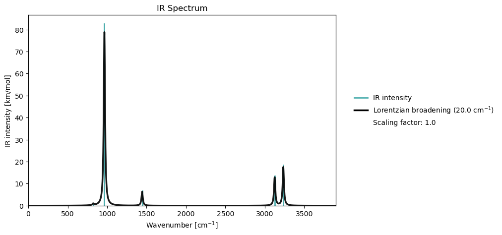
Once the vibrational analysis has been performed, we can animate the vibrational normal modes, or plot the IR spectrum.
vib_analysis.animate(vib_analysis_results, mode=1)
3Dmol.js failed to load for some reason. Please check your browser console for error messages.
vib_analysis.plot(vib_results=vib_analysis_results)