More birefringences & dichroisms

Faraday effect

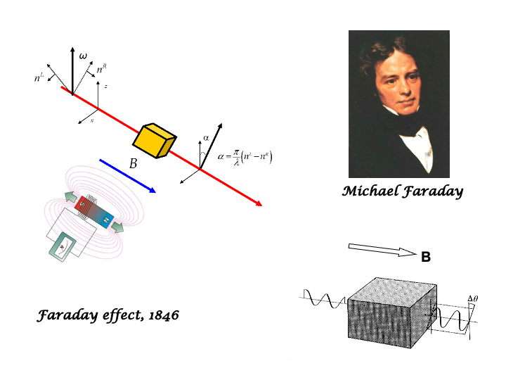
Observed in 1846, the Faraday effect is the rotation of the plane of polarization of a linearly polarized light beam traversing a transparent sample (glass, liquid, gas) occurring when a static magnetic field is applied with its direction parallel to that of propagating beam. Historically it was the first ever experimental evidence of a double refraction (birefringence) phenomenon, and in particular of a circular birefringence. It takes its name from the discoverer and it is also known an magnetic field induced-optical rotation. The rotation is proportional to the optical anisotropy, which depends linearly on the strength of the applied magnetic induction field. The mechanisms governing this effect involve the interaction of the static external magnetic induction field with the oscillating electric field of the light wave and with the electric multipoles of the sample. The term magnetic optical rotatory dispersion (MORD) is often used to denote the frequency dispersion of the Faraday effect, and thus of the corresponding circular birefringence.

For a fluid sample, the rotation with respect to the molecular frame is often given through the so-called Verdet constant \(V(\omega)\)

\[ \phi = V(\omega) B_z l\; \propto \; \omega \mbox{${\varepsilon}_{\alpha \beta \gamma}$} \big({\alpha^\prime}^{\rm B}_{\alpha\beta,\gamma}+\frac{1}{kT} \langle 0 |{\hat{m}}_\gamma|0 \rangle {\alpha^\prime}_{\alpha\beta}\big) B_z l, \]

where \(l\) is the path length and \({\alpha^\prime}^{\rm B}\) denotes the magnetic field derivative of \({\alpha^\prime}\), the antisymmetric electric dipole polarizability. The second term in the parentheses vanishes for closed-shell systems, as the magnetic dipole is in that case quenched, \( \langle 0 |{\hat{m}}_\gamma|0 \rangle = 0\).

The Verdet constant of a closed-shell system free of orbital degeneracies both in the ground and in the excited state, is therefore obtained from the response function/

\[ V(\omega) \propto i \omega {\varepsilon}_{\alpha \beta \gamma} \langle\langle \hat{\mu}_\alpha; \hat{\mu}_\beta, \hat{m}_\gamma \rangle\rangle_{\omega,0} \]

This contribution is sometimes referred to as the \(B\) term contribution to the Verdet constant. For molecules containing orbital degeneracies additional contributions arise (the \(A\) and \(C\) terms), in analogy with the closely related phenomenon - magnetic circular dichroism, see below.

Unit conversion factors for the Verdet constant are: 1 a.u. (rad\(\ e\ a_0\)\ \(\hbar^{-1}\)) =
\(8.03961 \times 10^{4}\) rad T\(^{-1}\) m\(^{-1}\) (SI) = 2.763816 \(\times 10^{2}\) min G\(^{-1}\) cm\(^{-1}\) (CGS).

Hypermagnetizabilities, Magnetic double refraction (Cotton-Mouton effect)

The Cotton-Mouton effect (CME) is a magnetic induction field-induced linear birefringence observed in the presence of a strong magnetic induction field \(\mathbf{B}\) with a component perpendicular to the direction of propagation of the beam. It is mainly due to the tendency of both the electric field associated with the light beam and the magnetic induction field to align the molecules exhibiting both an anisotropic electric dipole polarizability and an anisotropic magnetizability tensor (according to the Langevin-Born theory). The rearrangement of the electron density plays nevertheless a part through the mixed electric and magnetic hyperpolarizabilities, or hypermagnetizabilities.

The experimental quantity connected to the hypermagnetizability is the molar Cotton-Mouton constant \(_mC\). Semiclassically, for fluids composed of closed-shell systems

\[ _mC = \frac{2\pi N_A}{27}\left[\Delta\eta + Q\left(T\right)\right] \]

where \(\Delta\eta\) is the hypermagnetizability anisotropy

(53)\[\begin{eqnarray} \Delta\eta = \frac{1}{15}\left(3\eta_{\alpha\beta,\alpha\beta} - \eta_{\alpha\alpha,\beta\beta}\right), \end{eqnarray}\]

and

(54)\[\begin{eqnarray} Q\left(T\right) = \frac{1}{15kT}\left(3\alpha_{\alpha\beta}\xi_{\alpha\beta} - \alpha_{\alpha\alpha}\xi_{\beta\beta}\right), \end{eqnarray}\]

where \(\alpha\) is the (frequency-dependent) electric polarizability tensor, and \(\xi\) the magnetizability tensor. The two contributions to the molar Cotton–Mouton constant are therefore a temperature-independent term related to the hypermagnetizability \(\eta_{\alpha\beta,\gamma\delta}\) and a temperature-dependent molecular orientational part, the Langevin term.

When the magnetizability is expressed as a power series in the perturbing electric field

\[ {\xi}_{\alpha\beta}\left( \mathbf{F} \right) = \xi_{\alpha\beta} + \zeta_{\gamma,\alpha\beta} F_\gamma + \frac{1}{2} \eta_{\gamma\delta,\alpha\beta} F_\gamma F_\delta + ..., \]

the expansion coefficients \(\zeta_{\gamma,\alpha\beta}\) and \(\eta_{\gamma\delta,\alpha\beta}\) define the molecular first and second hypermagnetizability. The first indices of \(\zeta\) and \(\eta\) refer to the electric field and the last two to the magnetic field. In fluids, the experimentally measured property is related to the anisotropy of \(\eta\). From the expansion above it can be seen that the static hypermagnetizability \(\eta\) corresponds to the fourth derivative of the molecular energy

\[ \eta_{\alpha\beta,\gamma\delta} = -\left. \frac{\partial^{4} E\left( {{\mathbf F}},{{\mathbf B}}\right)} {\partial F_\alpha \partial F_\beta \partial B_\gamma \partial B_\delta} \right|_{{{\mathbf F}},{{\mathbf B}} = {\bf 0}} \]

It can also be expressed in terms of \(\xi \left( \mathbf{F} \right)\), the magnetizability dependent on \({\mathbf{F}}\)

\[ \eta_{\alpha\beta,\gamma\delta} = \frac{\partial^2 \xi_{\gamma\delta}}{\partial F_\alpha \partial F_\beta} \Big|_{{\mathbf{F}}=0} \]

or \(\alpha \left( {\mathbf{B}} \right)\), the polarizability dependent on \({\mathbf{B}}\)

\[ \eta_{\alpha\beta,\gamma\delta} = \frac{ \partial^2 \alpha(-\omega;\omega)_{\alpha\beta}}{\partial B_\gamma \partial B_\delta} \Big|_{ {\mathbf{B}} =0 } \]

and we have indicated in the latter equation that it holds also for the frequency-dependent polarizability.

The hypermagnetizability is given as a sum of paramagnetic and diamagnetic contributions

(55)\[\begin{eqnarray} \eta_{\alpha\beta,\gamma\delta} & = & \eta_{\alpha\beta,\gamma\delta}^{\rm para}(-\omega;\omega,0,0)+\eta_{\alpha\beta,\gamma\delta}^{\rm dia}(-\omega;\omega,0) \end{eqnarray}\]

corresponding to a sum of a cubic response and a quadratic response\index function

(56)\[\begin{eqnarray} \eta_{\alpha\beta,\gamma\delta}^{\rm para}(-\omega;\omega,0,0) & = & -\langle\langle \hat{\mu}_\alpha;\hat{\mu}_\beta,\hat{m}_\gamma, \hat{m}_\delta \rangle\rangle_{\omega,0,0}, \\ \eta_{\alpha\beta,\gamma\delta}^{\rm dia}(-\omega;\omega,0) & = & \langle\langle \hat{\mu}_\alpha;\hat{\mu}_\beta,\hat{\xi}^{{\rm B,B}}_{\gamma\delta} \rangle\rangle_{\omega,0} \end{eqnarray}\]

where the diamagnetic magnetizability operator in the second term is

\[ \hat{\xi}^{{\rm B,B}}_{\alpha \beta} = -2 {\hat{H}^{{\rm B,B}}}_{\alpha \beta} \]

We recall here that the magnetic dipole moment and diamagnetic magnetizability operators, and thus the partitioning of the hypermagnetizability into para- and diamagnetic components, may depend on the chosen gauge origin.

Finite field approaches were used in studies of magnetic double rifrangence. In these calculations \(\eta_{\alpha\beta,\gamma\delta}\) is obtained combining the available analytic linear response methods with the numerical finite difference approach. The frequency-dependent electric dipole polarizability can be computed in the presence of a magnetic induction field, and the hypermagnetizability is obtained by numerical differentiation. This approach in general requires complex algebra as the perturbation is purely imaginary, whereas most electronic structure codes use real wave functions. In the more often used finite field approach one computes the magnetizability \(\xi\) with and without an external electric field perturbation. However, in this approach only the static value of the required hypermagnetizability is obtained. Analytic calculations of the quadratic and cubic responses also including London orbitals to ensure gauge origin independence can nowadays be carried out. The effect of the London orbitals on improving the basis set convergence appears to be small.

For atoms, choosing the origin of the gauge at the nucleus automatically makes the dependence on the gauge vanish, and there is no advantage in using LAOs. Moreover, the evaluation of \(\Delta\eta\) may be reduced to the calculation of the Cauchy moments \(S(-2n)\) and of the dipole-dipole-quadrupole hyperpolarizability frequency dispersion coefficients.

Unit conversion factors for hypermagnetizability \(\eta\): 1 a.u. (\((e a_0^{2})^2 (e \hbar/{{m_{\mathrm e}}})^{2} {E_{\rm h}}^{-3})\) = 2.98425 \(\times 10^{-52}\) C\(^2\) m\(^2\) J\(^{-1}\) T\(^{-2}\) (SI) = 2.68211 \(\times 10^{-44}\) cm\(^3\) G\(^{-2}\) (CGS).

Electric-Field-Gradient-Induced Birefringence (Buckingham birefringence)

As a magnetic induction field can give rise to an optical anisotropy through its interaction with the anisotropic magnetizability of a molecule, so can an electric field gradient, through its coupling with a permanent molecular quadrupole moment. The corresponding birefringence is commonly called electric-field-gradient-induced
birefringence, more recently Buckingham birefringence, and it exhibits a linear dependence on the strength of the electric field gradient. Besides the orientational Langevin-Born-type effect, acting on quadrupolar molecules and due to both the electric field associated with the light wave and to the static external field gradient, it also involves the rearrangement of the electron density as a consequence of the electron interaction with the electric and magnetic wave vectors associated with the beam and with the externally applied electric field gradient. In this case mixed electric dipole, electric quadrupole and magnetic dipole hyperpolarizabilities play their role in determining the strength of the effect. Buckingham birefringence has been often employed for the determination of molecular quadrupole moments.

For an ideal gas at constant pressure, for light along the \(Z\) axis

(57)\[\begin{eqnarray} \Delta n & = & n_X - n_Y = \frac{N_A \nabla F}{15 V_m \epsilon_0} s = \frac{3 \nabla F}{2 V_m} {_mQ}(\omega,T), \\ _mQ(\omega,T) & = & \frac{2 N_A}{45 \epsilon_0} s \end{eqnarray}\]

where \(V_m\) is the molar volume, \(\nabla F\) is the external electric field gradient, arranged so that \(\nabla F =\nabla F_{XX} =-\nabla F_{YY}\) and \(\nabla F_{ZZ}=0\). T he above equation introduces the Buckingham constant \(_mQ\), which depends through the quantity \(s\) on the circular frequency of the light and on the temperature. For non-dipolar systems, where the quadrupole moment does not depend on the choice of origin,

\[ s = b\left(\omega\right) + \frac{1}{kT}\Theta_{\alpha\beta}\alpha_{\alpha\beta}\left(-\omega;\omega\right), \]

involving the molecular quadrupole moment \(\Theta_{\alpha\beta}\) and the frequency-dependent electric dipole polarizability \({{\alpha}_{\alpha\beta}}(-\omega;\omega)\). The temperature-independent contribution is

\[ b\left(\omega\right) = B_{\alpha\beta,\alpha\beta}\left(-\omega;\omega,0\right) - \mathcal{B}_{\alpha,\alpha\beta,\beta} \left(-\omega;\omega,0\right) - \frac{5}{\omega} \varepsilon_{\alpha\beta\gamma} J^\prime_{\alpha,\beta,\gamma}\left(-\omega;\omega,0\right) \]

and is a combination of three mixed hyperpolarizabilities

(58)\[\begin{eqnarray} B_{\alpha\beta,\gamma\delta}\left(-\omega;\omega,0\right) &=& \langle\langle\hat{\mu}_{\alpha};\hat{\mu}_\beta,\hat{\Theta}_{\gamma\delta}\rangle\rangle_{\omega,0},\\ \mathcal{B}_{\alpha,\beta\gamma,\delta}\left(-\omega;\omega,0\right) &=& \langle\langle\hat{\mu}_{\alpha};\hat{\Theta}_{\beta\gamma},\hat{\mu}_\delta\rangle\rangle_{\omega,0},\\ J'_{\alpha,\beta,\gamma}\left(-\omega;\omega,0\right) &=& i \langle\langle\hat{\mu}_{\alpha};\hat{m}_{\beta},\hat{\mu}_\gamma \rangle\rangle_{\omega,0}. \end{eqnarray}\]

The expressions are somewhat more complex for dipolar fluids, where the quadrupole moment becomes origin dependent. The formal expression for \(s\) does not change provided that we refer to a frequency-dependent origin for the quadrupole operator, commonly labelled as the effective quadrupole center. For any other choice of the origin we have

\[ s = b\left(\omega\right) + \frac{1}{kT}\left\{\Theta_{\alpha\beta}\alpha_{\alpha\beta}\left(-\omega;\omega\right)-\mu_\alpha\left[A_{\beta,\alpha\beta}\left(-\omega;\omega\right) + \frac{5}{\omega} \varepsilon_{\alpha\beta\gamma} G^\prime_{\beta\gamma}\left(-\omega;\omega\right)\right]\right\}. \]

The effective quadrupole center is defined as the point in space where the last term in this equation, involving the molecular dipole moment \(\mu_\alpha\) and the mixed polarizabilities

\(A_{\alpha,\beta\gamma}\left(-\omega;\omega\right)\) and \(G^\prime_{\alpha\beta}\left(-\omega;\omega\right)\), vanishes.

Magnetic circular dichroism

For a medium that is isotropic in the absence of magnetic fields, the Faraday \(A\), \(B\) and \(C\) terms determining the MCD of a transition from the electronic state \(|0\rangle\) to the electronic state \(|n\rangle\) are defined as

\[\begin{eqnarray*} A \left( 0 \rightarrow n \right) &=& \frac{1}{2} \left[ \left< n \left| \mathbf{m} \right| n \right> - \left< 0 \left| \mathbf{m} \right| 0 \right> \right] \cdot {\mathcal Im} \Big( \left< 0 \left| \boldsymbol{\mu} \right| n \right> \times \left< n \left| {\boldsymbol{\mu}} \right| 0 \right> \Big), \\ B \left(0 \rightarrow n \right) &=& {\mathcal Im} \Big\{ \sum_{k \neq 0} \frac{ \left< k | \mathbf{m}| 0 \right>} {\omega_{k0}} \cdot \left< 0 | \boldsymbol{\mu} |n \right> \times \left< n | \boldsymbol{\mu} | k \right> + \\ &\ & \sum_{k \neq n} \frac{\left<n|\mathbf{m}|k\right>} {\omega_{kn}}\cdot\left<0|\boldsymbol{\mu}|n\right>\times \left<k|\boldsymbol{\mu}|0\right>\Big\}, \\ C \left(0\rightarrow n\right) &=& \frac{1}{2} \left< 0 \left|\mathbf{m}\right|0\right> \cdot {\mathcal Im} \Big(\left< 0\left|\boldsymbol{\mu}\right|n\right> \times \left<n\left| \boldsymbol{\mu} \right|0\right> \Big), \end{eqnarray*}\]

where an average over the molecular orientations has been made. These tensors correspond to the single residues of the tensors that determine the Verdet constant of the Faraday effect. The \(A\) term exists only if either \(|0\rangle\) or \(|n\rangle\) is degenerate, whereas the \(C\) term is non-vanishing only if \(|0\rangle\) is degenerate.

The \(B\) terms exist in all cases, independently of the appearance of any ground- and excited-state degeneracies.
We can rearrange the equation for \(B\) above recalling that \((\hat{\mu}_{\alpha})_{lm}^{\ast} = (\hat{\mu}_{\alpha})_{lm}\),
\((\hat{m}_{\alpha})_{lm}^{\ast} = - (\hat{m}_{\alpha})_{lm}\) and \( {\mathcal Im} (z) = -i (z - z^{\ast})/2\), and we find that the \(B(0 \to n)\) term can be written in terms of a single residue of a quadratic response function as

(59)\[\begin{eqnarray} {B \left( 0\rightarrow n \right) = } i {\varepsilon}_{\alpha \beta \gamma} \Big( \lim_{\omega \rightarrow \omega_{n0}} \hbar (\omega - \omega_{n0}) \langle\langle \hat{\mu}_{\gamma};\hat{m}_{\beta},\hat{\mu}_{\alpha} \rangle\rangle_{0, \omega} \Big). \end{eqnarray}\]

By analogy to the spectral representation expression for the single residue we may also write

\[ \lim_{\omega \to \omega_{n0}} \hbar (\omega-\omega_{n0}) \langle\langle \hat{\mu}_{\gamma}; \hat{m}_{\beta}, \hat{\mu}_{\alpha} \rangle\rangle_{0,\omega} = M_{\mu_\alpha}^{0 \gets n} M_{m_\beta \mu_\gamma}^{n\gets 0}(0), \]

where \(M_{\mu_\alpha}^{0\gets n}\) and \(M_{m_\beta \mu_\gamma}^{n\gets 0}(0)\) indicate specific one- and (formally) two-photon transition matrix elements between state \(|0\rangle\) and state \(|n\rangle\), respectively.

Both the \(A\) and \(B\) terms come out directly from calculations using the complex polarization propagator approach [SRCN08].